Despite enormous progress, the frequently challenging task of correctly assigning the relative configuration of unknown chiral natural products can still not be fully automated. ^[1] Assignments are often based on NMR parameters such as scalar couplings and ROE/NOE‐derived distances, which can be used to find structures following well established procedures. ^[2] For anisotropic NMR data such as residual dipolar or quadrupolar couplings (RDCs and RQCs), or residual chemical shift anisotropies (RCSAs) this is less intuitive, as these parameters require structure models of the compounds under investigation. The experimental data has to be tested against parameters back‐calculated from these models, and configurational assignments are made based on minimal root mean‐square deviations (RMSD) or Q‐factors. ^[3]

However, estimating the certainty with which configurations are assigned rely on likelihood models like the akaike information criterion (AIC).[ ^1c , ^1d , ⁴ ] The AIC score represents the sum ${\chi }^2$ of squared violations of experimental and back‐calculated NMR parameters $\Delta X=X^{\mathrm{e}\mathrm{x}\mathrm{p}}-X^{\mathrm{c}\mathrm{a}\mathrm{l}\mathrm{c}}$ weighted by squared experimental errors ${\sigma }_X^2$ [Eq. 1], and amended by an additional penalty $k$ denoting the number of fitting parameters.

Back‐calculation of RDCs, RQCs, and RCSAs in the single‐conformer single‐tensor (SCST) approximation requires five independent fitting parameters for computing the alignment tensor, and the constant $k=5$ can be dropped from further considerations here. For independent observables $X_i$ with Gaussian‐distributed multiplicative probabilities (likelihoods) $p_i\sim \mathrm{e}\mathrm{x}\mathrm{p}(-1/2\Delta X_i^2/{\sigma }_X^2)$ , the sum ${\chi }^2\sim -\log (\prod p_i)\sim \sum \Delta X_i^2/{\sigma }_X^2$ represents the AIC log‐likelihood function, which should become minimal for the best‐fit molecular configuration assigned therefrom. The certainty or relative probability with which two diastereomers A and B can be differentiated is then given by their relative AIC weights $p_A/p_B$ as given in Equation 2.

Standard Monte‐Carlo (MC) based analysis of experimental errors yields distributions of AIC scores for alternate models, which can be used to compute quantitative estimates on diastereomeric differentiabilities.[ ^1c , ^1d , ⁴ , ⁵ ] Though this method is used frequently in the literature, we have observed that the back‐calculation of anisotropic NMR data subtly depends on the method from which the structure models were obtained (e.g. DFT functional and/or basis sets used). In a recent report we have demonstrated that even for simple molecules such as Isopinocampheol (IPC, 1), the inclusion of error estimates on the structure models themselves substantially lowers the certainties of RDC‐based configurational assignments from ≈1:10⁻¹¹ to 95 %:5 %. ^[5] For this, we have been criticized as to introducing “spurious structural noise” which “has to largely undermine discrimination capabilities of the AIC procedure”. ^[4] Unlike in our previous report ^[5] where structure uncertainties were estimated purely based on geometric considerations, we here would like to abandon this traditional classical approach entirely. Instead, we discuss a much more fundamental and quantum chemical source of “structural noise” that has not yet been evaluated with respect to RDC‐based configurational analysis, namely thermal vibrations.

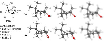
Though thermal motions are vastly faster than the NMR time‐scale and only time‐averaged expectation values are measured, any quantitative estimate on the probability with which two or more models can be distinguished by a given method has to consider structure fluctuations and thermal motions as well (Figure 1).

Figure 1

The differentiability of diastereomers not only depends on the quality of NMR data, but also on the “sharpness” with which a structure can be “seen”. For two diastereomers 1 a and 1 b of IPC depicted above (top and bottom row structure models), the time‐averaged expectation values of experimental data may appear unchanged. Yet the certainty with which both structures can be differentiated crucially depends on the “motion blur” and the “exposure time” of the experiment.

The average thermal mobility or positional uncertainty of atoms can be represented by anisotropic displacement parameters (ADPs, ellipsoids often referred to as Oak Ridge Thermal‐Ellipsoid Plot Program “orteps”), which are widely used in crystal structure analysis, but rarely have been applied to small organic molecules in the field of NMR crystallography, ^[6] and never been evaluated for solution‐state RDCs. The ADPs for $N$ atoms can be derived from the $3N\times 3N$ Hessian matrix $\mathbf{H}$ [Eq. 3] of mixed second derivatives of the electronic energy with respect to all atomic Cartesian coordinates, which can be obtained from quantum chemical DFT frequency calculations.

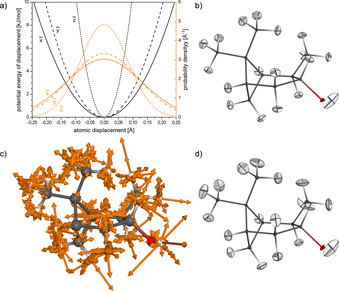
This matrix exactly represents the Cartesian force constants, which are also used for the calculation and interpretation of IR vibrational spectra. The atomic 3×3 sub‐matrices of the Hessian approximate a local three‐dimensional harmonic potential in which each atom moves independently. From the quantum chemical treatment of the harmonic oscillator in its ground state, this defines three orthogonal Gaussian probability distributions, which are narrower for large (stiff) force‐constants and steep potentials (Figure 2 a), and which can be represented as 3D ADP ellipsoids (Figure 2 b).

Figure 2

a) Harmonic potentials (black) and Gaussian‐type atomic displacement probability densities (orange) derived from the local harmonic oscillator approximation for H‐3 of IPC (1 a), where $\tilde{x}$ , $\tilde{y}$ , and $\tilde{z}$ denote the major axes (eigenvectors) of the ADP ellipsoid, and the squared standard deviations σ ² of displacement derived from the force‐constants are the corresponding eigenvalues ($k_{\tilde{x}}=$ 334, $k_{\tilde{y}}=$ 479, and $k_{\tilde{z}}=$ 2175 kJ mol⁻¹ Å⁻², and ${\sigma }_{\tilde{x}}=$ 0.132, ${\sigma }_{\tilde{y}}=$ 0.120, and ${\sigma }_{\tilde{z}}=$ 0.082 Å). b) Displacement ellipsoids set at the 2σ level (95.4 % probability) computed for IPC using the local approach. c) Superposition of normalized Cartesian displacement vectors (scaled by a factor of 2.5 for visualization) computed for all 81 vibration modes of IPC using the full Hessian matrix, and d) the 2σ ADPs computed therefrom (DFT B3LYP/6–311+G(2d,p)).

In real molecules, vibrational (stretch) and librational (angular bending) motions occur in correlated modes, and therefore models that are more accurate can be obtained diagonalizing the full Hessian. Vibrational and librational analysis then yields 3 N−6 fundamental modes for non‐linear molecules, along with the corresponding IR vibrational frequencies, the force‐constants, reduced masses, and atomic displacement vectors (Figure 2 c). Adding the atomic probability distributions along these displacement vectors also defines the ADPs as symmetric tensors corresponding to 3D trivariate Gaussian probability densities (Figure 2 d), which are similar to those obtained from the simpler local approach. A full description on the mathematics and the harmonic oscillator models is provided in the SI.

In the sequel, the ADPs calculated from the latter accurate approach are used, displaying standard deviations σ of thermal atomic displacements of approx. ±0.03–0.06 Å for non‐hydrogen atoms, and larger amplitudes of vibration for the hydrogen atoms in the direction of the bond vector (σ≈±0.08–0.09 Å, stiff bonds) or perpendicular (σ≈±0.12–0.19 Å, softer angle deformations) to it.

Now, vibrational ADPs are used in bootstrapping MC error analysis for the back‐calculation of RDCs from structure models. As RDCs depend on the time‐average $⟨1/r^3⟩$ of the distance between the coupling nuclei, the thermal motions introduce an error in the order of about ±1–3 % as compared to $1/r^3$ computed from static, non‐vibrating equilibrium structures of DFT optimized models. For various C−C‐H angles of IPC, thermal Gaussian distributions with typical standard deviations σ≈±5–7° are computed. ¹ D _CH RDCs also depend on the average orientation of the C−H bond vectors relative to the external NMR magnetic field, and the angles of C−H vectors relative to their equilibrium direction are approximately Rayleigh distributed (which is in fact the special case of combining two Gaussian distributions orthogonal to the C−H vector) with similar σ≈±5–7° (see the SI for plots of all distributions discussed here). These thermal angle fluctuations exceed by far the empirical estimates of σ≈±1.75° on structure uncertainties, which we have used previously to estimate diastereomeric differentiabilities. ^[5]

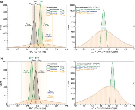
In Figure 3, MC distributions of two ¹ D _CH RDCs measured for 1 a in a typical polyarylacetylene LLC alignment medium ^[7] are shown. The experimental error for the measurement of the RDCs is estimated as σ _exp=±0.5 Hz, and the MC standard deviation σ _calc of RDCs back‐calculated for fixed static structures is similar in size. On the contrary, MC simulations using “fixed” experimental data (σ _exp set to zero) and only ADP based structure variations as described above, yield uncertainties on back‐calculated RDCs caused by thermal vibrations that are much larger with σ _vibr=±3.6 Hz. Propagation of Gaussian distributed errors adds up squared standard deviations, and the total error of back‐calculating RDCs becomes ${\sigma }_{\mathrm{t}\mathrm{o}\mathrm{t}\mathrm{a}\mathrm{l}}^2={\sigma }_{\mathrm{e}\mathrm{x}\mathrm{p}}^2+{\sigma }_{\mathrm{c}\mathrm{a}\mathrm{l}\mathrm{c}}^2+{\sigma }_{\mathrm{v}\mathrm{i}\mathrm{b}\mathrm{r}}^2$ . With ${\sigma }_{\mathrm{v}\mathrm{i}\mathrm{b}\mathrm{r}}^2\gg {\sigma }_{\mathrm{e}\mathrm{x}\mathrm{p}}^2+{\sigma }_{\mathrm{c}\mathrm{a}\mathrm{l}\mathrm{c}}^2$ , thermal vibrations are by far the most important source of uncertainty and almost exclusively dominate the orange curves in Figure 3, and this even applies to the allegedly very “rigid” structure of IPC. This also renders the somehow arbitrary estimate of σ _exp made in the first place nearly irrelevant.

Figure 3

Monte‐Carlo error analysis (100 000 steps) for C‐2/H‐2 (a) and C‐3/H‐3 (b) ¹ D _CH RDCs of IPC. The left plots show the simulated error of D ^exp (green curves, σ _exp=±0.5 Hz), and the corresponding error derived for D ^calc on the equilibrium structure of IPC (black curves, σ _calc≈±0.3 Hz). The very broad blue curve of RDC fluctuations originating solely from structure vibrations (σ _vibr) dominates the total uncertainty σ _total=±3.6 Hz of the back‐calculated RDCs (orange curves), and the blue curve is almost completely covered by the orange distribution. The plots on the right show the MC derived distributions of ΔD excluding (green curves) or including thermal vibrations (orange curves).

To account for all sources of errors in RDC evaluations, the ${\sigma }_X^2$ term in Equation (1) needs to be substituted by ${\sigma }_{\mathrm{t}\mathrm{o}\mathrm{t}\mathrm{a}\mathrm{l}}^2$ and therefore be expanded as stated in Equation 4, with ${\sigma }_{\mathrm{v}\mathrm{i}\mathrm{b}\mathrm{r}}^2$ being the decisive term in the denominator.

Using an experimental RDC data set measured for 1 a (11 ¹ D _CH RDCs as specified in the SI), and evaluating this data against structure models of the four IPC diastereomers 1 a–d, yields typical MC derived distributions of AIC scores as shown in Figure 4. In Figure 4 a, the uncorrected AIC scores cf. Equation (1) are plotted, whereas in Figure 4 b the vibration‐corrected [Eq. (4)] distributions are shown. Computing quantitative “diastereomeric differentiabilities” ^[5] according to Equation (2) now effectively measures the overlap of these distributions, and the larger their separation becomes, the more certain the correct configuration of IPC can be assigned from the lowest AIC scores. Using AICs on DFT optimized, static equilibrium structures, ^[4] the differentiability of 1 a vs. the alternate models 1 b–d is estimated to an exhilarating ratio of ≫1:e⁻²⁵⁰ (Figure 4 a). Applying the corresponding corrections emerging from thermal motions to the AIC scores reduces the differentiability of 1 a:1 b to 80.9 % and 18.9 %, respectively, and only 1 c and 1 d can be safely excluded as wrong configurations based on mismatching RDC data (Figure 4 b). Obviously, “structural noise” originating from thermal vibrations and the harmonic oscillator ground state model sets significant and natural upper limits to the discrimination capabilities of the AIC procedure which have gone unnoticed so far.

Figure 4

Distributions of a) uncorrected [Eq. (1)] and b) vibration‐corrected [Eq. (4)] AIC scores obtained from evaluating a RDC data set on four diastereomers 1 a–d of IPC (1 000 000 step MC simulations using σ _exp=±0.5 Hz, respectively). The distributions are labelled with their corresponding estimated diastereomeric differentiabilities (certainties of assignments), demonstrating that the certainty to identify the correct configuration 1 a (green curves) is dramatically reduced when considering vibrational broadening of RDCs.

At this point, it must be clearly pointed out not to confuse averages and uncertainties. The time‐averaged expectation values (i.e. the mean of the curves in Figure 3) are related to the quantity measured by NMR, and the average of ΔD is very close (Figure 3 a) or only slightly shifted (Figure 3 b) to what is calculated for static equilibrium structures. Though this is the foundation for all RDC‐based configurational assignments reported in the literature so far, statements on certainties with which these assignments are made must consider the breadth of the ΔD distributions.

Indeed, close inspection of the MC data shown in Figure 3 b for the C‐3/H‐3 RDC of 1 a and the corresponding ΔD, reveals that thermal averaging ^[8] even does slightly shift this RDC expectation value by about 2.6 Hz as compared to using a static model of 1 a. In the SI, we detail the mathematics of analytically estimating thermal corrections to average RDCs, based on the ADP tensor $\mathbf{U}$ (in units [Ų]) and the tensor $\mathbf{D}$ of mixed second derivatives (in units [Hz Å⁻²]) of RDCs with respect to Cartesian coordinates [Eq. 5].

Our preliminary results show that these corrections $⟨{\Delta D}_{\mathrm{v}\mathrm{i}\mathrm{b}\mathrm{r}}^{\mathrm{c}\mathrm{o}\mathrm{r}\mathrm{r}}⟩$ are frequently in the order of about ±5–10 %, and we continue to work on evaluating the significance of thermal vibrations and molecular flexibility for the process of back‐calculating RDCs.In general, most DFT methods seem to slightly overestimate the force constants computed—that is, bonds are calculated to be too “stiff”—and therefore, the frequencies are often scaled down before computing dependent thermochemical properties or comparing the vibrational frequencies with experimental data for example, from IR spectra (see SI). The ADPs scale inversely with the vibrational frequencies, and thus unscaled frequencies provide a lower bound to these thermal motions and also a lower bound to the structural uncertainties we would like to explore here. In addition, all derivations outlined above considered harmonic oscillators in their ground states only (zero‐point vibrations), which is a good approximation for most molecules at standard temperature. In excited states, the average mean squared displacements increase and scale with the quantum number n by (n+1/2), though in these cases anharmonic corrections may become increasingly important. Therefore, the considerations outlined here provide a lower bound on the average atomic displacement parameters (ADPs), and this in turn imposes an upper limit on the diastereomeric differentiability of structures based on NMR data such RDCs.

In the final consequence this result means that the differentiability of diastereomers based on comparisons between measured NMR‐parameters and back‐calculated parameters from structural models depends much more on the uncertainties of the calculated atomic positions than on experimental errors (unless they are exceedingly large). Due to the fact that these uncertainties are dominated by atomic vibrations, the ability to differentiate between diastereomers is restricted by first principles irrespective of the level of theory used to calculate the structures.

All calculations have been done with ConArch⁺, a program that is available free of charge from the authors.[ ⁵ , ^7c ]