Density estimation using deep generative neural networks

Qiao Liu, Jiaze Xu, Rui Jiang, Wing Hung Wong

Contributed by Wing Hung Wong, March 1, 2021 (sent for review January 7, 2021; reviewed by Faming Liang and Weijie Su)

Author contributions: Q.L., R.J., and W.H.W. designed research; Q.L. and W.H.W. performed research; Q.L. and J.X. contributed new reagents/analytic tools; Q.L. analyzed data; and Q.L., R.J., and W.H.W. wrote the paper.

Reviewers: F.L., Purdue University; and W.S., University of Pennsylvania.

https://doi.org/10.1073/pnas.2101344118, Volume: 118, Issue: 15, Pages: 1-6

Article Type: Research Article Article History

Publisher: National Academy of Sciences

- Facebook
- Twitter
- Linkedin
- Whatsapp
Altmetric

Table of Contents

Methods
Results
Discussion
Supplementary Material
Data Availability

Abstract

Density estimation is among the most fundamental problems in statistics. It is notoriously difficult to estimate the density of high-dimensional data due to the “curse of dimensionality.” Here, we introduce a new general-purpose density estimator based on deep generative neural networks. By modeling data normally distributed around a manifold of reduced dimension, we show how the power of bidirectional generative neural networks (e.g., cycleGAN) can be exploited for explicit evaluation of the data density. Simulation and real data experiments suggest that our method is effective in a wide range of problems. This approach should be helpful in many applications where an accurate density estimator is needed.

Density estimation is one of the fundamental problems in both statistics and machine learning. In this study, we propose Roundtrip, a computational framework for general-purpose density estimation based on deep generative neural networks. Roundtrip retains the generative power of deep generative models, such as generative adversarial networks (GANs) while it also provides estimates of density values, thus supporting both data generation and density estimation. Unlike previous neural density estimators that put stringent conditions on the transformation from the latent space to the data space, Roundtrip enables the use of much more general mappings where target density is modeled by learning a manifold induced from a base density (e.g., Gaussian distribution). Roundtrip provides a statistical framework for GAN models where an explicit evaluation of density values is feasible. In numerical experiments, Roundtrip exceeds state-of-the-art performance in a diverse range of density estimation tasks.

Keywords

deep learning, neural network, density estimation, importance sampling, GAN

License: CC BY

Liu,Xu,Jiang,and Wong: Density estimation using deep generative neural networks

Let $p (\cdot)$ be a density on a $n$ -dimensional Euclidean space $χ$ . The task of density estimation is to estimate $p (\cdot)$ based on a set of independently and identically distributed data points ${x_{i}}_{i = 1}^{N}$ drawn from this density.

Traditional density estimators such as histograms (1, 2) and kernel density estimators (KDEs) (3, 4) typically perform well only in low dimension. Recently, neural network-based approaches were proposed for density estimation and yielded promising results in problems with high-dimensional data points such as images. There are mainly two families of such neural density estimators: autoregressive models (5 6–7) and normalizing flows (8 9 10–11). Autoregression-based neural density estimators decompose the density into the product of conditional densities based on probability chain rule $p (x) = \prod_{i} p (x_{i} | x_{1 : i - 1})$ . Each conditional probability $p (x_{i} | x_{1 : i - 1})$ is modeled by a parametric density (e.g., Gaussian or mixture of Gaussian), of which the parameters are learned by neural networks. Density estimators based on normalizing flows represent $x$ as an invertible transformation of a latent variable $z$ with known density, where the invertible transformation is a composition of a series of simple functions whose Jacobian is easy to compute. The parameters of these component functions are then learned by neural networks.

As suggested in ref. 12, both of these are special cases of the following general framework. Given a differentiable and invertible mapping $G : R^{n} \to R^{n}$ and a base density $p_{z} (z)$ , the density of $x = G (z)$ can be represented using the change of variable rule as follows:

p_{x} (x) = p_{z} (z) {| det (J_{z}) |}^{- 1},

[1]

where

J_{z} = (\partial G (z)) / \partial z^{T}

is the Jacobian matrix of function

G (\cdot)

at point

z

. Density estimation at

x

can be solved if the base density

p_{z} (z)

is known and the determinant of Jacobian matrix is feasible to calculate. To achieve this, previous neural density estimators have to impose heavy constraints on the model architecture. For example, refs. , , and require the Jacobian to be triangular, ref. constructed low rank perturbations of a diagonal matrix as the Jacobian, and ref. proposed a circular convolution where the Jacobian is a circulant matrix. These strong constraints diminish the expressiveness of neural networks, which may lead to poor performance. For example, autoregressive neural density estimators based on learning

p (x_{i} | x_{1 : i - 1})

are naturally sensitive to the order of the features. Moreover, the change of variable rule is not applicable when the domain dimension in base density differs from target density. However, experiences from deep generative models [e.g., GAN () and VAE ()] suggested that it is often desirable to use a latent space of smaller dimension than the data space.

To overcome the limitations above, we propose a neural density estimator called Roundtrip. Our approach is motivated by recent advances in deep generative neural networks (15, 17, 18). Roundtrip differs from previous neural density estimators in two ways. 1) It allows the direct use of a deep generative network to model the transformation from the latent variable space to the data space, while previous neural density estimators use neural networks only to learn the parameters in the component functions that are used for building up an invertible transformation. 2) It can efficiently model data densities that are concentrated near learned manifolds, which is difficult to achieve by previous approaches as they require the latent space to have the same dimension as the data space. Importantly, we also provide methods, based on either importance sampling and Laplace approximation, for the pointwise evaluation of the density estimate. We summarize our major contributions in this study as follows: 1) We propose a general-purpose neural density estimator based on deep generative models, which requires less restrictive model assumptions compared to previous neural density estimators. 2) We show that the principle in previous neural density estimators can be regarded as a special case in our Roundtrip framework. 3) We demonstrate state-of-the-art performance of Roundtrip model through a series of experiments, including density estimation tasks in simulations as well as in real data applications ranging from image generation to outlier detection.

Methods

Method Overview.

The key idea of Roundtrip is to approximate the target distribution as a convolution of a Gaussian with a distribution induced on a manifold by transforming a base distribution where the transformation is represented by two GAN models (Fig. 1). After learning the weights of two GAN models by training on data, density estimation is achieved by an offline algorithm.

Fig. 1.

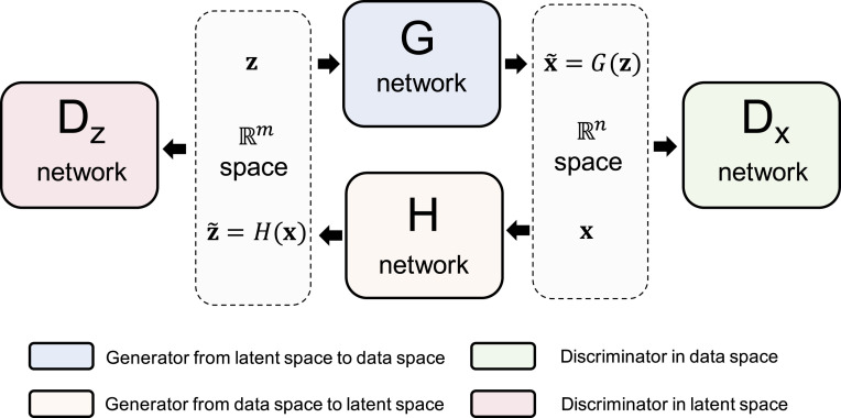
The overview of Roundtrip framework. In the latent space, latent variable $z$ follows a standard Gaussian distribution, which is fed to the $G$ network. The $H$ network maps $x$ from data space to the latent space. The $D_{x}$ network works as a discriminator for discerning the true data $(x)$ from the generated data $(\tilde{x})$ . The $D_{z}$ network is another discriminator for distinguishing the generated latent variable $(\tilde{z})$ from the real latent variable $(z)$ .

Model for the Data Density.

Consider two random variables $z \in R^{m}$ and $x \in R^{n}$ where $z$ has a known density $p_{z} (z)$ (e.g., standard Gaussian) and $x$ is distributed according to a target density $p_{x} (x)$ that we intend to estimate based on i.i.d. observations from it. We introduced two functions $G (\cdot)$ and $H (\cdot)$ for learning a forward and backward mapping relationship between the two distributions. These two functions are learned by two neural networks (Fig. 1). The bidirectional GAN architecture has been used by previous works (17, 19) for computer vision tasks, but here we intend to exploit it for a new task of density estimation. To do this, we denote $G (z) = \tilde{x}$ and $H (x) = \tilde{z}$ and assume that the forward mapping error follows a Gaussian distribution:

x = \tilde{x} + ε, ε_{i} \sim N (0, σ^{2}) .

[2]

Typically, we set $m < n$ , which means that $\tilde{x}$ takes values in a manifold of $R^{n}$ with intrinsic dimension $m$ . Basically, this roundtrip model utilizes $G (\cdot)$ to produce a manifold and then approximate the target density as a mixture of Gaussians where the mixing density is the induced density $p_{\tilde{x}} (\tilde{x})$ on the manifold. In what follows, we will set $p_{z} (z)$ to be a standard Gaussian $p_{z} (z) = {(\sqrt{2 π})}^{- m} \exp (- (1 / 2) {‖ z ‖}_{2}^{2})$ . Based on the model assumption from [2], we have $p_{x | z} (x | z) = {(\sqrt{2 π} σ)}^{- n} \exp (- (1 / 2 σ^{2}) {‖ x - G (z) ‖}_{2}^{2})$ . Then, the target density can be expressed as follows:

p_{x} (x) = \int p_{x | z} (x | z) p_{z} (z) d z = {(\frac{1}{\sqrt{2 π}})}^{m + n} σ^{- n} \int e^{- \frac{v (x, z)}{2}} d z,

[3]

where $v (x, z) = {‖ z ‖}_{2}^{2} + σ^{- 2} {‖ x - G (z) ‖}_{2}^{2}$ . The density estimation problem has been transformed to computing the integral in Eq. 3. Assuming that $G (\cdot)$ and $H (\cdot)$ have already been learned, we evaluate the integral in Eq. 3 by either importance sampling or Laplace approximation.

Importance Sampling.

The simplest way to estimate [3] is to use the empirical expectation by $(1 / N) \sum_{i = 1}^{N} p_{x | z} (x | z_{i})$ where $z_{i} \sim p_{z} (z)$ . However, this is usually extremely inefficient as $p_{x | z} (x | z)$ typically takes low values at most values of $z_{i}$ sampled from $p_{z} (z)$ . Thus, we propose to sample $z_{i}$ from an importance distribution $q (z)$ instead of the base density $p_{z} (z)$ and use the importance-weighted estimate:

p^{I S} (x) = \frac{1}{N} \sum_{i = 1}^{N} p_{x | z} (x | z_{i}^{q}) w (z_{i}^{q}),

[4]

where $N$ is the sample size, $w (z) = p_{z} (z) / q (z)$ is the importance weight function, ${z_{i}^{q}}_{i = 1}^{N}$ are i.i.d. samples from $q (z)$ . We propose to set $q (z)$ to be a Student t distribution with the center at $\tilde{z} = H (x)$ . This choice is motivated by the following considerations. 1) For a given $x$ , $p_{x | z} (x | z)$ is likely to be maximized at values of $z$ near $\tilde{z} = H (x)$ . 2) Student t distribution has a heavier tail than Gaussian which provides a control of the variance of the summand in Eq. 4. Thus, instead of directly evaluating [3] that only requires $G (\cdot)$ , we introduced an importance distribution $q (z)$ , where the center is determined by $H (\cdot)$ , to achieve a more efficient evaluation. More details including an illustrative example of importance sampling are provided in SI Appendix, Fig. S1.

Laplace Approximation.

We can also obtain an approximation to the integral in [3] by Laplace’s method. To achieve this goal, we expand $G (z)$ around $\tilde{z} = H (x)$ to obtain a quadratic approximation to $v (x, z)$ , which then leads to a multivariate Gaussian integral that is solvable in closed form. The full derivations are given in SI Appendix, Text S1. The resulting Laplace approximation for [3] is as follows:

p^{L P} (x) \approx {(\frac{1}{\sqrt{2 π}})}^{n} σ^{- n} \sqrt{det (Σ)} e^{- \frac{c (x)}{2}},

[5]

where $J_{\tilde{z}} \in ℝ^{n \times m}$ is the Jacobian of $G (z)$ at $\tilde{z}$ , $Σ = {(I + σ^{- 2} J_{\tilde{z}}^{T} J_{\tilde{z}})}^{- 1} \in ℝ^{m \times m}$ , $det (\cdot)$ denotes the determinant of a matrix, and $c (x) = {‖ H (x) ‖}_{2}^{2} + σ^{- 2} {‖ x - G (H (x)) ‖}_{2}^{2} - μ^{T} Σ^{- 1} μ$ . $(μ, Σ)$ are the parameters of a constructed multivariate Gaussian distribution. Interestingly, we note that the change of variable rule represented by [1] can be viewed as a special case of [5] if the following three conditions are satisfied. 1) $m = n$ . 2) $H (\cdot) = G^{- 1} (\cdot)$ . 3) $σ \to 0$ . The proof is given in SI Appendix, Text S2. Note that if $G (\cdot)$ and $H (\cdot)$ are approximated by neural networks, then their Jacobians are easy to compute and [5] can be evaluated numerically.

In the remaining part of Methods, we discussed how to learn $G (\cdot)$ and $H (\cdot)$ given observation data.

Adversarial Training Loss.

The Roundtrip model consists of a pair of two GAN models. In the forward GAN model, the network $G$ aims at generating samples ${\{{\tilde{x}}_{i}\}}_{i = 1}^{N}$ that are similar to observation data ${x_{i}}_{i = 1}^{N}$ while the discriminator $D_{x}$ tries to distinguish observation data (positive) from generated samples (negative). In the backward GAN model, the network $H$ and the discriminator $D_{z}$ aim to transform the data distribution to approximate the base distribution in latent space. Discriminators can be considered as (neural network-based) binary classifiers where the input data points will be asserted to be positive (1) or negative (0). The loss functions of the above four neural networks ( $G$ , $H$ , $D_{z}$ , and $D_{x}$ ) in the training process can be represented as the following:

{\begin{matrix} ℒ_{G A N} (G) = E_{z \sim p (z)} {(D_{x} (G (z)) - 1)}^{2} \\ ℒ_{G A N} (D_{x}) = E_{x \sim p (x)} {(D_{x} (x) - 1)}^{2} + E_{z \sim p (z)} D_{x}^{2} (G (z)) \\ ℒ_{G A N} (H) = E_{x \sim p (x)} {(D_{z} (H (x)) - 1)}^{2} \\ ℒ_{G A N} (D_{z}) = E_{z \sim p (z)} {(D_{z} (z) - 1)}^{2} + E_{x \sim p (x)} D_{z}^{2} (H (x)) \end{matrix},

[6]

where $z$ and $x$ are sampled in batches from base density $p (z)$ and data density $p (x)$ , respectively. In practice, sampling $x$ from data density $p (x)$ can be regarded as a procedure of randomly sampling from i.i.d. observations data with replacement. Minimizing the loss of a generator (e.g., $ℒ_{G A N} (G)$ ) and the corresponding discriminator (e.g., $ℒ_{G A N} (D_{x})$ ) are adversarial as the two networks ( $G$ and $D_{x}$ ) compete with each other during the training process. Note that the least-square loss functions we used in Eq. 6 were recommended by LSGAN (20).

Roundtrip Loss.

During the training, we also aim to minimize the roundtrip loss, which is defined as $ρ_{z} (z, H (G (z)))$ and $ρ_{x} (x, G (H (x)))$ , where $ρ_{z}$ , $ρ_{x}$ are distance functions and $z$ , $x$ are sampled from the base density $p_{z} (z)$ and the data density $p_{x} (x)$ , respectively. The principle is to minimize the distance when a data point goes through a roundtrip transformation between two data domains. If $m < n$ , this will ensure that $x \to H (x) \to G (H (x))$ will stay close to the projection of $x$ to the manifold induced by $G$ , and $z \to G (z) \to H (G (z))$ will stay close to $z$ . Since our model assumes Gaussian errors in [2], we use the L₂ distance for both $ρ_{z}$ and $ρ_{x}$ . This leads to the roundtrip loss:

ℒ_{R T} (G, H) = α {‖ x - G (H (x)) ‖}_{2}^{2} + β {‖ z - H (G (z)) ‖}_{2}^{2},

[7]

where $α$ and $β$ are two constant coefficients. The idea of roundtrip loss which exploits transitivity for regularizing structured data can also be found in refs. 17 and 19.

Full Training Loss.

Combining the adversarial training loss and roundtrip loss together, we get the full training loss for generator networks and discriminator networks as $ℒ (G, H) = ℒ_{G A N} (G) + ℒ_{G A N} (H) + ℒ_{R T} (G, H)$ and $ℒ (D_{x}, D_{z}) = ℒ_{G A N} (D_{x}) + ℒ_{G A N} (D_{z})$ , respectively. To achieve joint training of the two GAN models, we iteratively updated the parameters in the two generative models ( $G$ and $H$ ) and the two discriminative models ( $D_{z}$ and $D_{x}$ ), respectively. Thus, the overall iterative optimization problem in Roundtrip can be represented as follows:

G^{*}, H^{*}, D_{x}^{*}, D_{z}^{*} = {\begin{matrix} \arg \min_{G, H} ℒ (G, H) \\ \arg \min_{D_{x}, D_{z}} ℒ (D_{x}, D_{z}) \end{matrix} .

[8]

After an iterative model training process, the learned networks $G^{*}$ and $H^{*}$ will then be used as $G (\cdot)$ and $H (\cdot)$ functions in the density estimation procedure. The training can be monitored using the average log likelihood of the data in the validation set. We stop the training when there is no further improvement of the average log likelihood on the validation set.

Model Architecture.

The model architecture of Roundtrip is highly flexible. In most cases, when it is utilized for density estimation tasks with vector-valued data, we used fully connected layers for both generative networks and discriminative networks. Specifically, the $G$ network contains 10 fully connected layers and each layer has 512 hidden nodes, while the $H$ network contains 10 fully connected layers and each layer has 256 hidden nodes. The $D_{x}$ network contains four fully connected layers and each layer has 256 hidden nodes, while the $D_{z}$ network contains two fully connected layers and each layer has 128 hidden nodes. The leaky-ReLu activation function is deployed as a nonlinear transformation in each hidden layer.

Roundtrip can also handle tensor-valued data such as images. Similar to the model architecture in DCGAN (21), we used transposed convolutional layers for generating the image $G (z)$ from the latent vector $z$ , and traditional convolutional neural networks to get the latent representation $H (x)$ for the image $x$ . Note that Batch normalization (22) is applied after each convolutional layer or transposed convolutional layer (detailed hyperparameters were provided in SI Appendix, Table S3).

Labeled Data and Conditional Density Estimation.

We provide a strategy for conditional density estimation given labeled data. The original Roundtrip model is extended by one-hot encoding the class label $y$ as an additional input to both $G$ and $D_{x}$ networks in a conditional GAN (CGAN) manner (23). The label information will then be combined in the hidden representations in $G$ and $D_{x}$ networks by concatenation. Conditional density estimation is modeled as $p_{x | y} (x | y) = \int p_{x | y, z} (x | y, z) p_{z} (z) d z$ . After training on labeled data, Roundtrip is able to evaluate $p_{x | y} (x | y)$ given any test data and the label to condition on.

Note that for the image datasets (MNIST and CIFAR-10) used in our study, we regard the marginal distribution of $y$ as uniform distribution. i.e., we have $p (y = i) = \frac{1}{10}, i = 0,1, \dots, 9$ . Then the Bayesian posterior probability is calculated as $p (y = i | x) = (p (y = i) p (x | y = i) / p (x)) = (p (y = i) p (x | y = i) / \sum_{i} p (y = i) p (x | y = i))$ . Downstream tasks such as the image classification can be achieved by maximizing the posterior probability $\underset{i}{argmax} p (y = i | x)$ .

Results

Experiment Settings.

We test the performance of Roundtrip in a series of experiments, including simulation studies and real data studies. For the density estimation task, we compared our method to the widely used Gaussian KDE as well as several neural density estimators, including MADE (6), RealNVP (10), and MAF (7). For the outlier detection task, comparisons are also made to two commonly used outlier detection methods: one-class SVM (24) and Isolation Forest (25). Note that the default setting of Roundtrip was based on the importance sampling strategy. Results of Roundtrip density estimator based on Laplace approximation are reported in SI Appendix, Fig. S2.

The neural networks in Roundtrip model were implemented with TensorFlow (26). In all experiments, we set $α = 10$ and $β = 10$ in Eq. 7. For the parameter $σ$ in our model, we first pretrained the Roundtrip model for 20 epochs and selected $σ$ from ${0.01, 0.05, 0.1, 0.2, 0.4, 0.5}$ as the value that maximizes the average likelihood on validation test. Sample size $N$ in importance sampling is set to 40,000 as default. An Adam optimizer (27) with a learning rate of 0.0002 was used for backpropagation and updating model parameters. We stop model training when there is no improvement on the average log-likelihood in the validation set in 10 consecutive epochs.

We took Gaussian KDE as a baseline where the bandwidth is selected by Silverman’s “rule of thumb” (28) or Scott’s rule (29). We choose the one with better result to present. The three alternative neural density estimators (MADE, RealNVP, and MAF) were implemented using codes from https://github.com/gpapamak/maf. For outlier detection tasks, we implemented one-class SVM and Isolation Forest using Scikit-learn library (30), where the default parameters were used. To ensure fair model comparison, both simulation and real data were randomly split into a 90% training set and a 10% test set. For neural density estimators including Roundtrip, 10% of the training set was kept as a validation set. The image datasets with training and test set were directly provided which require no further data split.

Evaluation.

For simulation datasets with two dimensions, we directly visualized both true density and estimated density on a two-dimensional (2D) bounded region. For simulation datasets with higher dimensions where the true density can be calculated, we evaluate different density estimators by calculating the Spearman (rank) correlation between true density and estimated density based on the test set. For real data where the ground truth density is not available, the average estimated density (natural log-likelihood) on the test set will be considered as a metric for evaluation.

In the application of outlier detection, we measure performance by calculating the precision at k, which is defined as the proportion of correct results in the top-k ranks. We set k to the number of outliers in the test set.

Simulation Studies.

We first designed three 2D simulation datasets to test the performance of different neural density estimators where the truth density can be calculated.

a)Independent Gaussian mixture. $x_{i} \sim (1 / 3) (N (- 1, {0.5}^{2}) + N (0, {0.5}^{2}) + N (1, {0.5}^{2})), i = 1,2.$ Each dimension of this simulation dataset follows a Gaussian mixture distribution with three components.

b)Eight-octagon Gaussian mixture. $x \sim (1 / 8) \sum_{i = 1}^{8} N (μ_{i}, Σ_{i})$ where $μ_{i} = (3 \cos (π i / 4), 3 \sin (π i / 4))$ , and $Σ_{i} = [\begin{matrix} {cos}^{2} \frac{π i}{4} + {0.16}^{2} {sin}^{2} \frac{π i}{4} & (1 - {0.16}^{2}) \sin \frac{π i}{4} \cos \frac{π i}{4} \\ (1 - {0.16}^{2}) \sin \frac{π i}{4} \cos \frac{π i}{4} & {sin}^{2} \frac{π i}{4} + {0.16}^{2} {cos}^{2} \frac{π i}{4} \end{matrix}], i = 1, \dots, 8$ . This simulation dataset follows a Gaussian mixture distribution, where the two dimensions are conjuncted by the covariance matrix.

c)Involute. $x_{1} \sim N (r \sin (2 r), {0.4}^{2}), x_{2} \sim N (r \cos (2 r), {0.4}^{2})$ where $r$ follows a uniform distribution $U (0,2 π)$ . This simulation dataset shows a nonlinear distribution around an involute of a circle.

The 20,000 i.i.d. points were sampled from each of the above true data distribution. After model training, we directly estimated the density in a 2D bounded region ( $100 \times 100$ grid) with the different methods (Fig. 2). In cases a and b, Roundtrip clearly separates the components in the mixture while other neural density estimators either failed (MADE) or contain obvious trajectory between different components (RealNVP and MAF). In case c, the highly nonlinear structure in the density is captured by Roundtrip in a much more accurate manner than the other methods. To compare the methods in higher dimension, we took case a for a further study by increasing the dimension up to 10 (containing $3^{10}$ modes). Roundtrip still achieves a Spearman correlation of 0.829 at dimension 10, compared to 0.669 of RealNVP, 0.595 of MAF, and 0.14 of KDE (SI Appendix, Fig. S1). These results demonstrated the importance of using more expressive models, which allowed Roundtrip to represent complicated density forms that are hard to approximate by more restrictive neural density models.

Fig. 2.

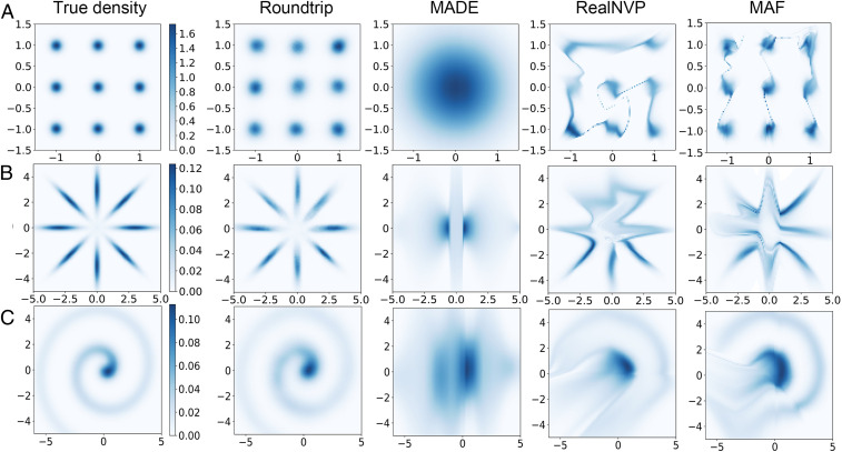
True density and estimated density by different neural density estimators (Roundtrip, MADE, RealNVP, and MAF) with three simulation datasets. Density plots were shown on a 100 × 100 grid 2D bounded region. True densities were shown in the first column. Each row gives results of a dataset: (A) independent Gaussian mixture; (B) eight-octagon Gaussian mixture; (C) Involute.

Real Data Studies.

University of California, Irvine, datasets.

We collected five datasets (AReM, CASP, HEPMASS, BANK, and YPMSD) from the University of California, Irvine (UCI) machine learning repository (31) with dimensions ranging from 6 to 90 and sample size from 42,240 to 515,345 (see more details about data description and data preprocessing in SI Appendix, Text S3). Unlike simulation data, these real datasets have no ground truth for the density. Hence, we evaluated different methods by calculating the average log-likelihood on the test set as suggested by previous work (7). Table 1 illustrates the performance of Roundtrip and the other neural density estimators. A Gaussian KDE fitted to the training data is also reported as a baseline. The results show that Roundtrip significantly outperforms other neural density estimators by achieving the highest average log-likelihood on the test set of each dataset.

Table 1.

Performance of different methods on five UCI datasets

	AReM	CASP	HEPMASS	BANK	YPMSD
KDE	6.26 ± 0.07	20.47 ± 0.10	−25.46 ± 0.03	15.84 ± 0.12	247.03 ± 0.61
MADE	6.00 ± 0.11	21.82 ± 0.23	−15.15 ± 0.02	14.97 ± 0.53	273.20 ± 0.35
RealNVP	9.52 ± 0.18	26.81 ± 0.15	−18.71 ± 0.02	26.33 ± 0.22	287.74 ± 0.34
MAF	9.49 ± 0.17	27.61 ± 0.13	−17.39 ± 0.02	20.09 ± 0.20	290.76 ± 0.33
Roundtrip	11.74 ± 0.04	28.38 ± 0.08	−4.18 ± 0.02	35.16 ± 0.14	297.98 ± 0.52

The average log likelihood and 2 SDs are shown. The best performance among five methods is shown in bold.

Image datasets.

Deep generative models have demonstrated their power in generating synthetic images. However, a conventional deep generative model alone cannot provide quality scores for generated images. Here, we propose to use our Roundtrip method to generate both the image and its quality score based on the density of the image. We test this approach on two commonly used image datasets, MNIST (32) and CIFAR-10 (33), where in each of these datasets, the image comes from 10 distinct classes. Roundtrip model was modified by introducing an additional class label $y$ to both $G$ and $D_{x}$ network and convolutional layers were used in $G$ , $H$ , and $D_{x}$ (Methods). We then model the conditional density estimation by $p_{x | y} (x | y) = \int p_{x | y, z} (x | y, z) p_{z} (z) d z$ where $y \sim Cat (10)$ denotes a categorical distribution with 10 distinct classes. The class label $y$ will be one-hot encoded before feeding to the model. We use this modified Roundtrip model to simultaneously generate images conditional on a class label and compute the within-class density of the image. The other neural density estimators typically require a lot of tricks, including rescaling pixel values to $[0,1]$ , transforming the bounded pixel values into an unbounded logit space, and adding uniform noise, to achieve image generation and density estimation. In contrast, Roundtrip did not require additional transformation except for rescaling. In Fig. 3, the generated images of each class were sorted by decreased likelihood. It is seen that images generated by Roundtrip are more realistic than those generated by MAF (which is the best among alternative neural density estimators; see Fig. 2 and Table 1). Furthermore, the density provided by Roundtrip seems to correlate well with the quality of the generated images.

Fig. 3.

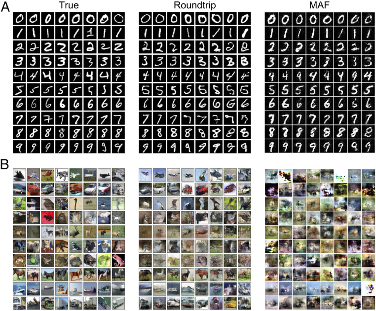
True images and generated images from Roundtrip and MAF models trained on MNIST and CIFAR-10 databases. Each row denotes the true or generated images of a specific class. (A) True and generated images of MNIST. (B) True and generated images of CIFAR-10. Images generated by Roundtrip and MAF are sorted by decreased likelihood for each class.

As a more systematic and quantitative comparison of the different methods for image data, we use the estimated conditional densities of a test image (conditional on label values) to obtain Bayesian predictions of the label (Methods). Roundtrip achieves the highest test accuracy on both MNIST and CIFAR-10 datasets (SI Appendix, Fig. S3). For example, on the MNIST dataset, Roundtrip gives a test accuracy of 0.983, compared to 0.911 of MADE, 0.744 of RealNVP, and 0.926 of MAF, which again demonstrates the superiority of Roundtrip.

Outlier detection.

Finally, we applied Roundtrip to an outlier detection task, where a data point with a very low density value is regarded as likely to be an outlier. We tested this method on three outlier detection datasets (Shuttle, Mammography, and ForestCover) from ODDS database (34).

Each dataset is split into training, validation, and test set (details of data description can be found in SI Appendix, Text S4). Besides the neural density estimators, we also provide comparisons with two baseline methods, namely one-class SVM (24) and Isolation Forest (25). The results shown in Table 2 were based on the average precision of three independent runs of each algorithm. The performance of Roundtrip is either the best or tied for the best for each dataset. For the ForestCover dataset, where the outlier percentage is very low (0.9%), Roundtrip achieves a precision of 17.7% while the precision of other neural density estimators is less than 6%. Roundtrip’s performance is robust to the choice of the sample size used in importance sampling (SI Appendix, Fig. S4A). As for computational efficiency, Roundtrip is more efficient in training but less efficient in testing, compared to the other neural density estimators (SI Appendix, Fig. S4B).

Table 2.

The precision at k of different methods on three ODDS datasets

	OC-SVM	I-Forest	RealNVP	MAF	Roundtrip
Shuttle	0.953	0.956	0.784	0.929	0.959
Mammography	0.037	0.482	0.474	0.407	0.482
ForestCover	0.127	0.058	0.054	0.046	0.177

The best performance among five methods is shown in bold.

Discussion

We propose Roundtrip as a general-purpose neural density estimator based on deep generative models. Unlike prior studies that focus on modeling the invertible transformation between a base density and the target density, where the parameters of the component functions are learned by neural networks, Roundtrip allows the direct use of a deep generative network to model the transformation from the latent variable space to the data space. In contrast to the change of variable rule used by previous methods, which requires equal dimension in the base density and the target density, Roundtrip provides a more flexible transformation between the base density and target density. In numerical experiments, Roundtrip outperforms previous neural density estimators in a variety of density estimation tasks, including simulation/real data studies and an outlier detection application.

Given the observed data, density estimation aims to recover the underlying density while deep generative modeling aims to generate new data similar to the observed ones. Our work provides a way to leverage the power of deep generative models for an accurate evaluation of density values.

Acknowledgements

The work of W.H.W. was supported by the NSF Grants (DMS1811920 and DMS195238). The work of R.J. was supported by the National Key Research and Development Program of China Grant (2018YFC0910404) and the National Natural Science Foundation of China Grants (61873141, 61721003, and 61573207). Q.L. and J.X. were supported by a China Scholarship Council scholarship.

The authors declare no competing interest.

This article contains supporting information online at https://www.pnas.org/lookup/suppl/doi:10.1073/pnas.2101344118/-/DCSupplemental.

Data Availability

Source code and data for Roundtrip are freely available on Zenodo repository (DOI: 10.5281/zenodo.3747161) (35) and (DOI: 10.5281/zenodo.3747144) (36). All data in this study are included in the article and/or supporting information. Previously published data were used for this work (https://archive.ics.uci.edu/ml/datasets/Activity+Recognition+system+based+on+Multisensor+data+fusion+%28AReM%29, https://archive.ics.uci.edu/ml/datasets/Physicochemical+Properties+of+Protein+Tertiary+Structure, https://archive.ics.uci.edu/ml/datasets/HEPMASS, https://archive.ics.uci.edu/ml/datasets/Bank+Marketing, https://archive.ics.uci.edu/ml/datasets/YearPredictionMSD, odds.cs.stonybrook.edu/, http://yann.lecun.com/exdb/mnist/, and https://www.cs.toronto.edu/∼kriz/cifar.html).

References

D. W. Scott, On optimal and data-based histograms. Biometrika 66, 605–610 (1979).

G. Lugosi, A. Nobel, Consistency of data-driven histogram methods for density estimation and classification. Ann. Stat. 24, 687–706 (1996).

M. Rosenblatt, Remarks on some nonparametric estimates of a density function. Ann. Math. Stat. 27, 832–837 (1956).

E. Parzen, On estimation of a probability density function and mode. Ann. Math. Stat. 33, 1065–1076 (1962).

B. Uria, M.-A. Côté, K. Gregor, I. Murray, H. Larochelle, Neural autoregressive distribution estimation. J. Mach. Learn. Res. 17, 7184–7220 (2016).

M. Germain, K. Gregor, I. Murray, H. Larochelle, “Made: Masked autoencoder for distribution estimation” in International Conference on Machine Learning, F. Bach, D. Blei, Eds. (JMLR, 2015), pp. 881–889.

G. Papamakarios, T. Pavlakou, I. Murray, “Masked autoregressive flow for density estimation” in Advances in Neural Information Processing Systems, U. von Luxburg, I. Guyon, S. Bengio, H. Wallach, R. Fergus, Eds. (Curran Associates, Inc., Red Hook, NY, 2017), pp. 2338–2347.

D. Rezende, S. Mohamed, “Variational inference with normalizing flows” in International Conference on Machine Learning, F. Bach, D. Blei, Eds. (JMLR, 2015), pp. 1530–1538.

J. Ballé, V. Laparra, E. P. Simoncelli, Density modeling of images using a generalized normalization transformation. arXiv [Preprint] (2015). https://arxiv.org/abs/1511.06281 (Accessed 27 October 2019).

L. Dinh, J. Sohl-Dickstein, S. Bengio, Density estimation using real nvp. arXiv [Preprint] (2016). https://arxiv.org/abs/1605.08803 (Accessed 3 November 2019).

A. Grover, M. Dhar, S. Ermon, “Flow-gan: Combining maximum likelihood and adversarial learning in generative models” in Proceedings of the AAAI Conference on Artificial Intelligence, J. Furman, G. Marchant, H. Price, F. Rossi, Eds. (Association for Computing Machinery, New York, NY, 2018).

D. P. Kingma., Improved variational inference with inverse autoregressive flow. Adv. Neural Inf. Process. Syst. 29, 4743–4751 (2016).

R. van den Berg, L. Hasenclever, J. M. Tomczak, M. Welling, Sylvester normalizing flows for variational inference. arXiv [Preprint] (2018). https://arxiv.org/abs/1803.05649 (Accessed 5 November 2019).

M. Karami, L. Dinh, D. Duckworth, J. Sohl-Dickstein, D. Schuurmans, “Generative convolutional flow for density estimation” in Workshop on Bayesian Deep Learning NeurIPS 2018, S. Bengio, H. M. Wallach, H. Larochelle, K. Grauman, N. Cesa-Bianchi, Eds. (Curran Associates, Inc., Red Hook, NY, 2018).

I. Goodfellow., “Generative adversarial nets” in Advances in Neural Information Processing Systems, Z. Ghahramani, M. Welling, C. Cortes, N. D. Lawrence, K. Q. Weinberger, Eds. (MIT Press, Cambridge, MA, 2014), pp. 2672–2680.

D. P. Kingma, M. Welling, Auto-encoding variational bayes. arXiv [Preprint] (2013). https://arxiv.org/abs/1312.6114 (Accessed 13 October 2019).

J.-Y. Zhu, T. Park, P. Isola, A. A. Efros, “Unpaired image-to-image translation using cycle-consistent adversarial networks” in Proceedings of the IEEE International Conference on Computer Vision, K. Ikeuchi, Ed. (IEEE, 2017), pp. 2223–2232.

A. Makhzani, J. Shlens, N. Jaitly, I. Goodfellow, B. Frey, Adversarial autoencoders. arXiv [Preprint] (2015). https://arxiv.org/abs/1511.05644 (Accessed 10 November 2019).

Z. Yi, H. Zhang, P. Tan, M. Gong, “Dualgan: Unsupervised dual learning for image-to-image translation” in Proceedings of the IEEE international conference on computer vision, K. Ikeuchi, Ed. (IEEE, 2017), pp. 2849–2857.

X. Mao., “Least squares generative adversarial networks” in Proceedings of the IEEE International Conference on Computer Vision, K. Ikeuchi, Ed. (IEEE, 2017), pp. 2794–2802.

A. Radford, L. Metz, S. Chintala, Unsupervised representation learning with deep convolutional generative adversarial networks. arXiv [Preprint] (2015). https://arxiv.org/abs/1511.06434 (Accessed 2 November 2019).

S. Ioffe, C. Szegedy, “Batch normalization: Accelerating deep network training by reducing internal covariate shift” in Proceedings of the 32nd International Conference on Machine Learning, B. Francis, B. David, Eds. (JMLR, 2015), pp. 448–456.

M. Mirza, S. Osindero, Conditional generative adversarial nets. arXiv [Preprint] (2014). https://arxiv.org/abs/1411.1784 (Accessed 3 November 2019).

B. Schölkopf, J. C. Platt, J. Shawe-Taylor, A. J. Smola, R. C. Williamson, Estimating the support of a high-dimensional distribution. Neural Comput. 13, 1443–1471 (2001).

F. T. Liu, K. M. Ting, Z.-H. Zhou, “Isolation forest” in 2008 Eighth IEEE International Conference on Data Mining, F. Giannotti, Ed. (IEEE, 2008), pp. 413–422.

M. Abadi., “Tensorflow: A system for large-scale machine learning” in 12th USENIX Symposium on Operating Systems Design and Implementation (OSDI 16), K. Keeton, T. Roscoe, Eds. (USENIX, 2016), pp. 265–283.

D. Kingma, J. Ba, Adam: A method for stochastic optimization. arXiv [Preprint] (2014). https://arxiv.org/abs/1412.6980 (Accessed 12 April 2017).

B. W. Silverman, Density Estimation for Statistics and Data Analysis (CRC Press, 1986), vol. 26.

D. W. Scott, Multivariate Density Estimation: Theory, Practice, and Visualization (Wiley, 2015).

F. Pedregosa., Scikit-learn: Machine learning in Python. J. Machine Learn. Res. 12, 2825–2830 (2011).

A. Asuncion, D. Newman, UCI machine learning repository (2007). https://archive.ics.uci.edu/. Accessed 13 December 2019.

Y. LeCun, C. Cortes, The MNIST database of handwritten digits (2010). http://yann.lecun.com/exdb/mnist/. Accessed 17 November 2019.

A. Krizhevsky, G. Hinton, Learning multiple layers of features from tiny images (2009). https://www.cs.toronto.edu/∼kriz/learning-features-2009-TR.pdf. Accessed 5 November 2019.

S. Rayana, ODDS Library. Outlier detection datasets. http://odds.cs.stonybrook.edu. Accessed 10 January 2020.

Q. Liu, J. Xu, R. Jiang, W. H. Wong, Code: Density estimation using deep generative neural network. Zenodo. 10.5281/zenodo.3747161. Deposited 25 February 2021.

Q. Liu, J. Xu, R. Jiang, W. H. Wong, Datasets: Density estimation using deep generative neural network. Zenodo. 10.5281/zenodo.3747144. Deposited 10 April 2020.