
Contributed by Thomas J. Sargent, March 3, 2021 (sent for review December 10, 2020; reviewed by Mariacristina De Nardi, Xavier Gabaix, and Benjamin Moll)
Author contributions: T.J.S., N.W., and J.Y. designed research; T.J.S., N.W., and J.Y. performed research; T.J.S. and N.W. analyzed data; and T.J.S., N.W., and J.Y. wrote the paper.
Reviewers: M.D.N., University of Minnesota; X.G., Harvard University; and B.M., London School of Economics and Political Science.
1T.J.S., N.W., and J.Y. contributed equally to this work.
Forces that shape wealth inequality are intermediated through an individual’s nonfinancial earnings growth rate g
As measured by Gini coefficients, fractile inequalities, and tail power laws, wealth is distributed less equally across people than are labor earnings. We study how luck, attitudes that shape saving decisions, and growth rates of labor earnings balance each other in ways that simultaneously shape joint distributions across people of labor earnings, age, and wealth together with an equilibrium rate of return on savings that plays a pivotal role in balancing contending forces. Strong motives for people to save and for firms to demand capital raise an equilibrium interest rate enough to make wealth grow faster than labor earnings. That makes cross-sectional wealth more unevenly distributed and have a fatter tail than labor earnings, as in US data.
We begin with a streamlined setting, in which an equilibrium interest rate and distribution of wealth depend on preferences and opportunities in a continuous-time economy populated by a unit measure of ex ante identical, but ex post heterogeneous, agents who have random life spans. After isolating forces that generate wealth inequality, we investigate how adding sources of ex ante heterogeneity alters equilibrium wealth distributions.* Our model makes cross-sectional wealth more unequal and fatter-tailed than labor earnings, as is true in US data.
A person is born at age 0 and dies at a random nonnegative age that is exponentially distributed with a constant death rate per unit of time, as in ref. 5. An agent ranks consumption processes by
As in refs. 5 and 6, we assume that people can purchase an actuarially fair “reverse-life-insurance” contract that provides payments at rate of until death in exchange for agreeing to transfer end-of-life wealth to an insurance company.
A random variable if an agent is alive, and otherwise. For (), wealth evolves as
A person can dissave when savings are positive, but cannot borrow against future labor earnings, i.e.,
We complete our model as did ref. 1 by letting a representative firm operate a Cobb–Douglas production technology. A representative firm operates a production function , where , , is the aggregate capital stock, and is aggregate labor demand. Physical capital depreciates at a constant rate . The firm rents capital and labor in competitive markets. The firm’s optimization problem implies that a competitive equilibrium interest rate and wage index satisfy:
Across people, random deaths are statistically independent. To sustain a constant population, we replenish the economy with new people born at a constant rate per unit of time. By a law of large numbers, the insurance company always breaks even by using its receipts to cover its payments to living annuity owners. In equilibrium, capital demand equals capital supply:
In equilibrium, labor demand equals labor supply: . The wage index equals an average wage rate across all agents so that . Because aggregate labor cost equals aggregate labor earnings, a law of large numbers† implies
Eqs. 4, 5, and 6 imply that the equilibrium interest rate and wage rate received by an agent with average labor efficiency satisfy
We provide analytic formulas to isolate forces that determine equilibrium outcomes.‡.
To assure existence of equilibrium objects, we assume
Labor earnings grow according to , and length of life is the only source of heterogeneity across people. Along with Condition [10], a constant mortality rate implies that the cumulative distribution function (CDF) of the cross-section of earnings is
Eq. 11 implies the following Lorenz curve of labor earnings:
By using Eq. 14, we obtain the following formula for the Gini coefficient of labor earnings:
A scalar
A person’s age is tied to her earnings by , and wealth at age satisfies
Inequality [23] also implies that the growth rate of consumption exceeds the growth rate of earnings, a consequence of a constant MPC out of total wealth and the existence of stationary equilibrium. Since inequality [23] holds, Eq. 22 implies that wealth is a convex function of earnings. That shape amplifies wealth inequality relative to earnings inequality.
Cross-section wealth is less equally distributed and has a fatter tail than nonfinancial earnings because individuals’ optimal saving choices make their financial wealth always grow at a faster rate than nonfinancial earnings. Younger people own less financial wealth, so they choose to make their wealth grow at faster rates than do older people. Growth rates of wealth still exceed growth rates of nonfinancial earnings for very old people. The higher growth rate of total wealth than of nonfinancial earnings combines with compound interest to widen the wealth distribution and fatten its right tail relative to earnings.
The inverse function presented in Eq. 22 is increasing in under Condition [23]. In a stationary equilibrium, those who live longer have higher earnings and more wealth. Indeed, the CDF of wealth, which we denote by , satisfies , which implies
Unlike the cross-section earnings distribution that satisfies a power law over the entire support of , the cross-section wealth distribution satisfies a power law only in the limit as . Thus, the fraction of wealth owned by the top percent that goes to the top percent of people, which we denote by , obeys
Inequality [23] and Eq. 26 together imply that : Cross-section wealth has a fatter right tail than earnings since the power-law exponent of cross-section wealth is smaller than the exponent of cross-section earnings.
In Appendix, we derive the following formula for the Lorenz curve of wealth:
Fig. 1 illustrates the mechanism that generates a fatter-tailed distribution for cross-section wealth than for earnings. Fig. 1 A and B show that earnings grow at a constant rate that is lower than the consumption growth rate . This occurs because grows at a nonlinear rate greater than consumption and earnings growth rates. While the growth rate of wealth decreases with age after starting from at , increases with age.

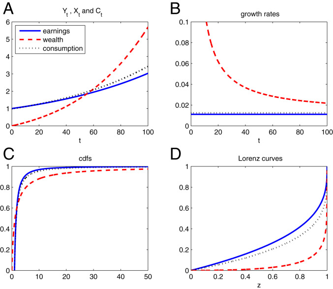
Earnings, wealth, and consumption: micro dynamics and macro cross-section distribution. A plots the levels of , , and . B plots the corresponding growth rate of change over time: , , and . C plots the CDFs of , , and . D plots the equilibrium stationary cross-section Lorenz curves for , , and . Parameter values are , , , , , , , and .
Fig. 1C plots cross-section distributions of , , and . Fig. 1D plots corresponding Lorenz curves. CDFs for both earnings and consumption are described globally by power laws having different exponents. Because our agents prefer to smooth consumption over time, it may at first appear surprising that the distribution of consumption is fatter-tailed than the distribution of earnings. But Condition [23] reveals that, in equilibrium, consumption grows faster than earnings. The distribution of wealth is not globally Pareto as earnings and consumption are, but instead approaches the shape of a Pareto distribution with the same power-law exponent as consumption as . Fig. 1D shows that wealth has a substantially steeper/convex Lorenz curve than consumption, which, in turn, has a steeper/convex Lorenz curve than earnings does. Consequently, the Gini coefficient for is larger than it is for consumption , which is larger than it is for labor earnings .
Note that the Gini coefficient, Lorenz curve, and tail fatness all provide the same inequality rankings for cross-section consumption, labor earnings, and wealth. Such identical rankings won’t prevail after we add ex ante heterogeneity across agents.
In a stationary equilibrium, . Summing over the wealth dynamics given in Eq. 2 across all agents and using a law of large numbers, we obtain the following relation for aggregate variables:
We have National Income and Product Accounts typical of models in the ref. 123–4 tradition:
To compute a stationary equilibrium interest rate, take the firm’s first-order conditions for capital and labor, and , and then substitute [13] and [25] for and , respectively, to obtain
This string of equalities implies a quadratic equation that restricts the stationary equilibrium :
To isolate sources of new findings about the equilibrium wealth distribution that our model brings, we purposefully choose consensus parameter values from the literature. Thus, we set commonly used values and an annual discount rate . We set preference and production function parameters to values used by refs. 1718–19. Following refs. 20 and 21, we set the capital share of national income, , to 0.36. We set an annual depreciation rate of capital, , to to match an estimate of the US depreciation-output ratio reported by ref. 22. We want an aggregate capital-output ratio equal to three, as in refs. 18 and 23, which, in light of Eq. 7, leads to an equilibrium interest rate of 6% per annum, as in refs. 17 and 18. Along with refs. 8 and 18 and others, we interpret the equilibrium risk-free rate in our model as a broad measure of average returns on capital. This is why we calibrate an annual (real) risk-free rate to be approximately 6%. We set the productivity parameter to 0.9, so that the wage rate for an agent with the average labor efficiency equals unity (a normalization). We set in order to set an agent’s expected lifetime at years, as in ref. 23.
In Table 1, we conduct a comparative static exercise with respect to the earnings growth rate . In addition to the equilibrium interest rate , we report Gini coefficients for earnings and wealth ( and ), power-law exponents ( and ) for the tail, and fractal inequalities ( and ) for the tail.

| , % | |||||||
| 5.88 | 0 | 0.58 | 3.79 | 0.10 | 0.18 | ||
| 6.60 | 0.18 | 0.72 | 3.34 | 2.08 | 0.20 | 0.30 | |
| 7.34 | 0.43 | 0.87 | 1.67 | 1.43 | 0.40 | 0.50 | |
| 7.77 | 0.63 | 0.95 | 1.29 | 1.21 | 0.59 | 0.68 |
Y and X are the Gini coefficients for cross-section earnings and wealth, respectively. For all levels of , the power-law exponent for earnings is , and the power-law exponent for wealth approaches as .
First, consider a case with . There is zero cross-section earnings inequality (hence, , , and ). An equilibrium interest rate that exceeds the annual rate of time preference makes young people want to save. Our analytical formulas indicate that wealth has a power-law exponent of , a Gini coefficient of , and fractal inequality for all . The fraction of wealth earned by the top % of people that goes to the top % is 18%, which, because it is larger than 10%, indicates that wealth is fat-tailed.
The (first) row in Table 1 shows that, in equilibrium, the pure life-cycle savings motive for young people, all of whom are born with no (or small) wealth, can generate a fat-tailed wealth distribution, even when their labor earnings are perfectly equal and wealth inequality is entirely driven by how long different agents live.
At a given interest rate , a higher labor-earnings growth rate strengthens incentives to borrow against future income to finance current consumption. To encourage savings and clear the asset market, the equilibrium must increase with . Also, as increases, (aggregate) labor becomes more productive, which raises firms’ demand for capital because capital and labor are complements.
Thus, as increases from 0 to 1%, cross-section earnings inequality increases because older people have higher earnings: The Gini coefficient for cross-section earnings increases from zero to , and the earnings tail becomes fatter (with the power-law exponent decreasing from to ). As a result, the fraction of earnings received by the top % of agents that goes to the top 0.1% equals 40%: , a fraction whose excess over 10% indicates substantial earnings inequality among the earnings-rich.
In order to elicit saving, the equilibrium interest rate increases from 5.88% to 7.34%. When , the return on savings is greater than when because the equilibrium interest rate is higher. As a result, cross-section wealth inequality increases substantially. The Gini coefficient for wealth increases to 0.87 from 0.58; the wealth tail becomes fatter with the power-law exponent decreasing to from 3.79; and the fraction of wealth owned by the top % of agents owned by the top % increases to from 18%.
Finally, if we adjust parameters to make the Gini coefficient of earnings equal 0.63, the value reported in refs. 18 and 23, we obtain . In this case, the annual equilibrium interest rate is 7.77%, and the wealth Gini coefficient is 0.95, significantly higher than its value of 0.78 in the US data. What makes cross-section wealth that much fatter-tailed than earnings is that the equilibrium interest rate is high and so many agents live so long, or, if we reinterpret the mortality parameter as partly measuring intergenerational bequest motive, that they care so much about their descendants. Ref. 8 analyzes a setup like this. See their p. 7 discussion on “finite lives and stochastic altruism” and their online appendix B.1.3. Enriching the mortality specification would allow us to improve fits here.††.
Table 1 confirms two insights about sources of wealth inequality. First, a higher growth rate of earnings increases Gini coefficients and fattens right tails of both earnings and wealth. Second, for all levels of , wealth inequality is larger than earnings inequality, whether we measure them with Gini coefficients (), power-law exponents for right tails (), or fractal inequalities (). This occurs because older people are both earnings-rich and wealth-rich; their voluntary savings makes their wealth grow at a faster rate than their earnings.‡‡ However, the result that wealth has a fatter tail than earnings may not hold when there is ex ante heterogeneity.
Table 1 confirms that the equilibrium interest rate exceeds the earnings growth rate .§§ The mechanism here is related to, but distinct from, one posited by ref. 27, which sees an condition as the fulcrum that creates wealth inequality. Unlike ref. 27, our model with its ex post heterogeneous agents explicitly incorporates equilibrium consumption responses of the type analyzed in refs. (123–4). Despite the action of the impatience parameter in making them prefer to front-load their consumption profiles, agents accept upward-sloping consumption profiles that fit together with an equilibrium age-dependent wealth growth rate that is larger than , which, in turn, exceeds the earnings growth rate . These outcomes prevail because, in equilibrium, an individual’s wealth accumulates at a rate higher than earnings.
Ref. 28 documents that ex ante heterogeneity influences equilibrium wealth distributions. Ref. 29 shows how positing different discount rates across agents can help match equilibrium wealth distributions. We can extend our baseline model to allow for this and other varieties of ex ante heterogeneity. Thus, suppose that groups of people, and , differ in earnings growth rates ( and ) , elasticity of intertemporal substitution ( and ), subjective discount rates ( and ), or death (or dynasty exit rates) and . Let denote the population of type- agents and denote the population of type- agents. Assume and , so that stationary earnings distributions exist for both groups.
The CDF for cross-section earnings is
Let
Consider the case where
The CDF or cross-section wealth for type is
The CDF of the cross-section wealth distribution is
Average wealth is
Next, we turn to a situation in which one group of agents is financially constrained:
Recall that for all agents in group and that their mass is . People in group all have positive savings. Therefore, the CDF for the wealth distribution has positive probability mass at : and
Equilibrium average wealth is
The equilibrium interest rate satisfies the following restriction:
In Tables 2 and 3, we display consequences of varying . We hold all other parameters at the same values for the two groups: , , and . When the subjective discount rate is just slightly larger than , which means holds (case 1), the equilibrium consumption rules for both groups are linear in wealth and earnings. We report these results in Table 2. The first row corresponds to the baseline case with no heterogeneity as . Therefore, , and we reproduce results from Table 1. By increasing (e.g., to 5.4%) and keeping , type- agents increase their consumption, and firms would want more capital if were fixed at 7.5%, so the equilibrium interest rate has to increase (to 7.65%). As a result, a higher interest rate helps savers accumulate wealth, and, hence, wealth inequality widens, as indicated by a higher Gini coefficient , a lower power-law exponent , and a higher fractional inequality .
| , % | |||||||
| 7.50 | 0.50 | 0.90 | 1.51 | 1.34 | 0.46 | 0.56 | |
| 7.59 | 0.50 | 0.91 | 1.51 | 1.29 | 0.46 | 0.60 | |
| 7.65 | 0.50 | 0.97 | 1.51 | 1.26 | 0.46 | 0.62 |
and are the Gini coefficient, and are the power-law exponents of the right tail, and and are the fractal inequality of the right tail for cross-section earnings and wealth, respectively.We set , , , , , , and .
| , % | |||||||
| 7.67 | 0.50 | 0.97 | 1.51 | 1.25 | 0.46 | 0.63 | |
| 7.67 | 0.50 | 0.97 | 1.51 | 1.25 | 0.46 | 0.63 |
and are the Gini coefficient, and are the power-law exponents of the right tail, and and are the fractal inequality of the right tail for cross-section earnings and wealth, respectively. We set , , , , , , and .
As we continue to increase to 5.45% (the first row in Table 3), consumption for group continues to increase up to the point where , which implies for all agents in group at . As a result, for markets to clear, the interest rate again continues to increase. Using [42], we confirm this intuition: the equilibrium interest rate: . Because the interest rate increased only 2 basis points as we increase from 5.4% to 5.45%, wealth inequality increases only slightly. Finally, further increasing does not change equilibrium outcomes because type- agents are constrained. This is why the two rows in Table 3 are the same.
Outcomes displayed in Tables 2 and 3 corroborate results of ref. 29, which uses heterogeneous discount rates to generate an empirically plausible wealth distribution.
Tables 4 and 5 reports equilibrium consequences of varying . We keep other parameters identical for the two groups: , , and . When the earnings growth rate is not too high so that holds (case 1), equilibrium consumption rules for agents in both groups are linear in wealth and earnings. We report these results in Table 4. The first row corresponds to the baseline case with no heterogeneity as and, thus, , and we recover results reported in Table 1. By increasing (e.g., to 1.3%) and keeping , type- agents increase their consumption, and firms would demand more capital (if were fixed at 7.5%), so the equilibrium interest rate has to increase (to 7.67%). As a result, savers accumulate wealth at a higher interest rate, and wealth inequality widens, as witnessed by a higher Gini coefficient , a lower power-law exponent , and a higher fractional inequality
| , % | |||||||
| 7.50 | 0.50 | 0.90 | 1.51 | 1.34 | 0.46 | 0.56 | |
| 7.57 | 0.53 | 0.91 | 1.39 | 1.30 | 0.52 | 0.59 | |
| 7.67 | 0.56 | 0.94 | 1.28 | 1.25 | 0.60 | 0.63 |
and are the Gini coefficients, and are the power-law exponents of the right tail, and and are the fractal inequality of the right tail for cross-section distribution for earnings and wealth, respectively. We set , , , , , , and .
| , % | |||||||
| 7.78 | 0.60 | 0.97 | 1.20 | 1.20 | 0.68 | 0.68 | |
| 7.88 | 0.64 | 0.97 | 1.11 | 1.16 | 0.79 | 0.73 | |
| 8.06 | 0.68 | 0.98 | 1.04 | 1.09 | 0.91 | 0.82 |
and are the Gini coefficients, and are the power-law exponents of the right tail, and and are the fractal inequality of the right tail for cross-section distribution for earnings and wealth, respectively. We set , , , , , , and .
As we increase to 1.39% (the first row in Table 5), consumption for group increases up to where , which implies for all agents in group at . As a result, for markets to clear, the interest rate again has to increase. Using [42], we confirm this reasoning: the equilibrium interest rate: . Earnings inequality and wealth inequality both also increase.
As we further increase from 1.39 to 1.6%, consumption for agents in group no longer responds, as they are involuntarily constrained to be hand-to-mouth consumers for any satisfying . As labor becomes more productive (higher ), the firm’s demand for capital continues to increase (as capital and labor are complements). In equilibrium, the interest rate rises to 8.06% to restore equilibrium for the case where .
A faster earnings growth rate increases both earnings inequality and the equilibrium interest rate . Therefore, wealth inequality increases because savers accumulate wealth at a faster rate via a higher . Thus, faster earnings growth generates larger earnings inequality and also larger wealth inequality. These outcomes are consistent with our baseline analysis with ex ante identical agents.
While inequality measures for earnings and wealth both increase with , whether wealth inequality is greater than earnings inequality for a given depends on how we measure inequality. When in equilibrium, the Gini coefficient (i.e., two times the area between the 45° line and the Lorenz curve) and measures of tail fatness (e.g., the power-law exponent and the fractal inequality, FI) yield opposite answers.
Table 5 shows that the earnings distribution has a fatter right tail than does the wealth distribution when in equilibrium. For example, when , the power-law exponent for earnings is 1.04, which is lower than the power-law exponent for wealth, 1.09. The fraction of wealth owned by the top percent owned by the top percent of people as goes to zero, , approaches 82%, which is already very large. However, this fractal inequality measure for earnings yields an even worse earnings inequality, , meaning that the fraction of earnings earned by the top percent that goes to the top percent of people as goes to zero, , which is larger than that measure for the wealth distribution.
Nevertheless, the Gini coefficient for earnings is much smaller than the Gini coefficient for wealth: versus for the case where . This is because group agents are at the bottom of the wealth distribution, with zero wealth, which substantially increases the Gini coefficient for wealth, while their being at the left tail evidently has no effect on the right tail of the wealth distribution. Indeed, the wealth-rich are people who have lower earnings growth, but who have lived long.
In Fig. 3, we plot the Lorenz curves for earnings and wealth in A and B, respectively. We see that as we increase , Lorenz curves for both earnings and wealth become steeper, and the Gini coefficient also increases.
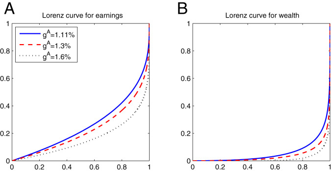
Lorenz curves for cross-section earnings (A) and wealth (B). We set , , , , , , and .
Our paper shares topics, but not models, methods, or findings, with ref. 27. Ref. 27 bristles with fascinating claims about sources of wealth inequalities and presents them to a broad audience by deploying what ref. 32 called “implicit theorizing” that can leave a technically inclined reader not knowing assumptions that make things fit together. Parts of his argument that lead him to emphasize an “” condition as a cause of cross-section dispersion in wealth rest on an appeal to a single-agent growth model that has no wealth or income inequality.
Our model tightly links outcomes for individuals to macroeconomic outcomes that include the celebrated “ and ” variables that concerned ref. 27. A wedge between an equilibrium growth rate for wealth/savings, and an earnings growth rate at the level of individual people (not at the aggregate level) makes cross-section wealth more unequal than labor earnings.
Mathematics ties together equilibrium model outcomes: The same forces that make cross-section wealth more unevenly distributed and fatter-tailed than cross-section earnings also make an individual’s wealth grow at a higher rate than do her earnings. Firms’ demand for physical capital and an equilibrium growth rate for an individual’s savings that exceeds the growth rate of her labor earnings () imply that the equilibrium interest rate exceeds the nonstochastic augmented golden-rule interest rate .
Our paper shares tools, explicit theorizing, and some, but not all, goals with ref. 8, but differs in focus and details of the formal economic environments being modeled. They study effects of technical change and automation on an equilibrium wealth distribution and derive power laws like ones that we, too, find. Details about insurance arrangements and whether earnings processes are stationary or display growth differ between their framework and ours. What unites our project and theirs is our common reliance on the same mathematical tools for characterizing outcomes in heterogeneous-agent models cast in continuous time in closed forms.*** .
To obtain an enlightening and interpretable explicit solution for the wealth distribution, we have analyzed an admittedly unrealistic model with no shocks to labor earnings. Uninsurable shocks to labor earnings are, of course, important, so in ref. 25, we incorporate permanent uninsurable Brownian shocks to labor earnings. Quantitative outcomes in that model depend crucially on earnings growth volatility and precautionary savings. That model can be used to study how government tax and transfer policies affect equilibrium outcomes.
The Kolmogorov Forward equation for the density function is
Since the total wealth at the stochastic death moment , we can rewrite [21] as follows for :
We thank Jess Benhabib, Alberto Bisin, Patrick Bolton, Mariacristina De Nardi, Xavier Gabaix, Fatih Guvenen, Dirk Krueger, Ye Li, Erzo Luttmer, Benjamin Moll, Jonathan Payne, Alexis Toda, and seminar participants at Columbia University and Shanghai Finance Forum for helpful criticisms.
All study data are included in the article.
1
2
3
4
5
6
7
8
9
10
11
12
13
14
15
16
17
18
19
20
21
22
23
24
25
26
27
28
29
30
31
32
33
34
35
36
 Earnings growth and the wealth distribution
 Facebook
 Twitter
 Linkedin
 Whatsapp


![The quadratic function Ψ(r) given in Eq. 34. The equilibrium interest rate satisfies Ψ(r*)=0 and (ρ+γg)<r*<(ρ+γλ) when λ>g≥0, as assumed in Condition [10].](/dataresources/secured/content-1766060224627-14235530-a2b7-4a40-b80d-69604846c7a7/assets/pnas.2025368118fig02.jpg)