
Edited by Marlan O. Scully, Texas A&M University, College Station, TX, and approved October 19, 2020 (received for review May 27, 2020)
Author contributions: N.J.C. designed research; and N.J.C. and M.G.J. performed research, derived the formulas, discussed the results, and wrote the paper.
We uncover an unsuspected quantum interference mechanism, which originates from the indistinguishability of identical bosons in time. Specifically, we build on the Hong–Ou–Mandel effect, namely the “bunching” of identical bosons at the output of a half-transparent beam splitter resulting from the symmetry of the wave function. We establish that this effect turns, under partial time reversal, into an interference effect in a quantum amplifier that we ascribe to time-like indistinguishability (bosons from the past and future cannot be distinguished). This hitherto unknown effect is a genuine manifestation of quantum physics and may be observed whenever two identical bosons participate in Bogoliubov transformations, which play a role in many facets of physics.
The celebrated Hong–Ou–Mandel effect is the paradigm of two-particle quantum interference. It has its roots in the symmetry of identical quantum particles, as dictated by the Pauli principle. Two identical bosons impinging on a beam splitter (of transmittance 1/2) cannot be detected in coincidence at both output ports, as confirmed in numerous experiments with light or even matter. Here, we establish that partial time reversal transforms the beam splitter linear coupling into amplification. We infer from this duality the existence of an unsuspected two-boson interferometric effect in a quantum amplifier (of gain 2) and identify the underlying mechanism as time-like indistinguishability. This fundamental mechanism is generic to any bosonic Bogoliubov transformation, so we anticipate wide implications in quantum physics.
The laws of quantum physics govern the behavior of identical particles via the symmetry of the wave function, as dictated by the Pauli principle (1). In particular, it has been known since Bose and Einstein (2) that the symmetry of the bosonic wave function favors the so-called bunching of identical bosons. A striking demonstration of bosonic statistics for a pair of identical bosons was achieved in 1987 in a seminal experiment by Hong, Ou, and Mandel (HOM) (3), who observed the cancellation of coincident detections behind a 50:50 beam splitter (BS) when two indistinguishable photons impinge on its two input ports (Fig. 1A). This HOM effect follows from the destructive two-photon interference between the probability amplitudes for double transmission and double reflection at the BS (Fig. 1B). Together with the Hanbury Brown and Twiss effect (4, 5) and the violation of Bell inequalities (6, 7), it is often viewed as the most prominent genuinely quantum feature: it highlights the singularity of two-particle quantum interference as it cannot be understood in terms of classical wave interference (8, 9). It has been verified in numerous experiments over the last 30 y (see, e.g., refs. 101112–13), even in case the single photons are simultaneously emitted by two independent sources (1415–16) or within a silicon photonic chip (17, 18). Remarkably, it has even been experimentally observed with He metastable atoms, demonstrating that this two-boson mechanism encompasses both light and matter (19).


(A) If two indistinguishable photons (represented in red and green for the sake of argument) simultaneously enter the two input ports of a 50:50 BS, they always exit the same output port together (no coincident detection can be observed). (B) The probability amplitudes for double transmission (Left) and double reflection (Right) precisely cancel each other when the transmittance is equal to 1/2. This is a genuinely quantum effect, which cannot be described as a classical wave interference. (C) The correlation function exhibits an HOM dip when the time difference between the two detected photons is close to zero (i.e., when they tend to be indistinguishable).
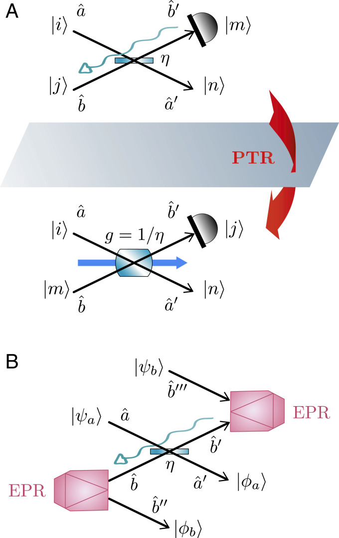
Here, we explore how two-boson quantum interference transforms under reversal of the arrow of time in one of the two bosonic modes (Fig. 2A). This operation, which we dub partial time reversal (PTR), is unphysical but nevertheless central as it allows us to exhibit a duality between the linear optical coupling effected by a BS and the nonlinear optical (Bogoliubov) transformation effected by a parametric amplifier. As a striking implication of these considerations, we predict a two-photon interferometric effect in a parametric amplifier of gain 2 (which is dual to a BS of transmittance 1/2). We argue that this unsuspected effect originates from the indistinguishability between photons from the past and future, which we coin “time-like” indistinguishability as it is the partial time-reversed version of the usual “space-like” indistinguishability that is at work in the HOM effect.
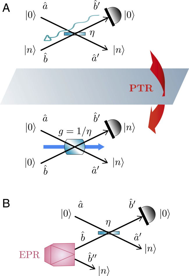
(A) BS under PTR, flipping the arrow of time in mode . The PTR duality is illustrated when photons impinge on port (with vacuum on port ), and we condition on all photons being reflected. The retrodicted state of mode (initially the vacuum state ) back propagates from the detector to the source (suggested by a wavy arrow). This yields the same transition probability amplitude (up to a constant) as for a PDC of gain with input state and output state . PDC is an active Bogoliubov transformation, requiring a pump beam (represented in blue). Note that the PTR duality is rigorously valid when this pump beam is of high intensity (i.e., treated as a classical light beam) since the Hamiltonian of Eq. 4 holds in this limit only. (B) Operational view of the PTR duality. As noted in ref. 20, if we prepare the entangled (EPR) state and send mode in the BS, we get the output state , which is precisely the two-mode squeezed vacuum state produced by PDC when the signal and idler modes are initially in the vacuum state.
Since Bogoliubov transformations are ubiquitous in quantum physics, it is expected that this two-boson interference effect in time could serve as a test bed for a wide range of bosonic transformations. Furthermore, from a deeper viewpoint, it would be fascinating to demonstrate the consequence of time-like indistinguishability in a photonic or atomic platform as it would help in elucidating some heretofore overlooked fundamental property of identical quantum particles.
The HOM effect is a landmark in quantum optics as it is the most spectacular manifestation of boson bunching. It is a two-photon intrinsically quantum interference effect where the probability amplitude of both photons being transmitted cancels out the probability amplitude of both photons being reflected. A 50:50 BS effects the single-photon transformations (for details, see Materials and Methods, Gaussian Unitaries for a BS and PDC)
Bogoliubov transformations on two bosonic modes comprise passive and active transformations. The BS is the fundamental passive transformation, while parametric down conversion (PDC) gives rise to the class of active transformations (also called nondegenerate parametric amplification). Although the involved physics is quite different (a simple piece of glass makes a BS, while an optically pumped nonlinear crystal is needed to effect PDC), the Hamiltonians generating these two unitaries are amazingly close, namely
The underlying concept of PTR will be formalized in Eq. 7, but we first illustrate this duality between a BS and PDC with the simple example of Fig. 2A, where photons impinge on port of a BS (with vacuum on port ), resulting in the binomial output state
These examples reflect the existence of a general duality between a BS and PDC. Indeed, as demonstrated in Materials and Methods, Proof of PTR Duality, partial transposition in Fock basis gives rise to PTR duality
The notion of time reversal can be conveniently interpreted using the so-called “retrodictive” picture of quantum mechanics (21). Along this line, PTR must be understood here as the fact that the “retrodicted” state of mode propagates backward in time, while the state of mode normally propagates forward in time (this is made precise in Materials and Methods, Retrodictive Picture of Quantum Mechanics). As shown in Fig. 2B, the PTR duality can be made operational by sending half of a so-called Einstein–Podoslky–Rosen (EPR) entangled state on mode , so that we access the output retrodicted state on the second entangled mode .
Due to this duality, the HOM effect for a BS of transmittance 1/2 immediately suggests the possible existence of a related interferometric suppression effect in a PDC of gain 2, namely . This striking prediction can indeed be verified by examining the state at the output of a PDC of gain (see Two-Photon Interference in a BS and PDC):
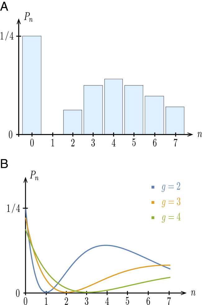
(A) Probability of observing photon pairs at the output of a PDC of gain when a single photon impinges on both the signal and idler input ports. The output state has a vanishing component, owing from two-photon interferometric suppression. The significant components are the vacuum as well as the terms with 2 to 10 pairs (the next terms quickly decay to zero). (B) Corresponding distributions of the photon pair number for a gain (showing a dip at ) and (showing a dip at ). The distributions are shown as continuous curves in order to guide the eye, but only integer values of are relevant. The curve for is also plotted for comparison.
The dependence of the probability of detecting a single pair () on the gain of PDC is given by (see Two-Photon Interference in a BS and PDC)
The origin of the two-boson quantum interference effect that we predict can be traced back to boson indistinguishability, similarly as for the HOM effect albeit in a time-like version (involving bosons from the past and future). We first recall that the HOM effect originates from what can be viewed as space-like indistinguishability (Fig. 4, Upper). When two photons impinge on a BS of transmittance , each photon has a probability amplitude of being transmitted, so the double-transmission amplitude is . In contrast, the probability amplitude of reflection is but with opposite signs for the two photons, so the double-reflection amplitude is . Since a double-transmission event is indistinguishable from a double-reflection event, we must add probability amplitudes, leading to . The double-transmission and double-reflection amplitudes exactly cancel out for , which originates from the fact that an exchange of the two indistinguishable photons in space (which turns a double-transmission into a double-reflection event) cannot lead to any observable consequence.
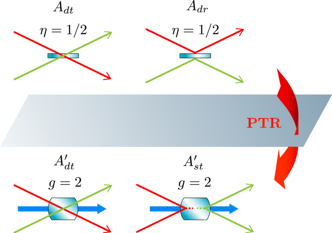
The HOM effect (Upper) is due to space-like indistinguishability: the double-transmission path (of amplitude ) where the two photons are transmitted interferes destructively with the double-reflection path (of amplitude ) where the two photons are reflected. Exchanging the two photons in space leads to the HOM effect in a BS of transmittance . According to PTR duality (by reversing the arrow of time in the second mode; Lower), the two interfering paths in a PDC correspond to the double-transmission event associated with amplitude (the two photons simply cross the PDC) and double-stimulated event of amplitude (the input photon pair is up converted into the pump beam, and another pump photon is down converted into a new photon pair). Exchanging the photon pairs in time induces a time-like interferometric suppression in a PDC of gain .
We now argue that it is the exchange of indistinguishable photons in time that is responsible for the interference effect in an amplifier (Fig. 4, Lower). When two photons impinge on a PDC with gain , they can be both transmitted without triggering a stimulated event, which is dual to the double transmission in a BS (where is substituted by ). Hence, the double-transmission amplitude in a PDC is . Another possible path giving rise to the coincident detection of two single photons is the combination of the stimulated annihilation and emission of a pair of photons, which is dual to the double reflection in a BS. This double-stimulated event admits a probability amplitude , where the minus sign results from the fact that the probability amplitude that the input pair disappears by stimulated annihilation and the probability amplitude that a new pair is created by stimulated emission have opposite signs. Again, since the double-transmission and double-stimulated events are indistinguishable, we must add their probability amplitudes and get , which vanishes when . Roughly speaking, we cannot know whether the “old” photons have been replaced by “new” photons or have been left unchanged, which we dub time-like indistinguishability.
The role of time reversal in quantum physics has long been a fascinating subject of questioning (see, e.g., ref. 22 and references therein), but the key idea of the present work is to consider a bipartite quantum system (two bosonic modes) with counterpropagating times. Incidentally, we note that the notion of time reversal has been exploited in the context of defining separability criteria (23, 24), but this seems to be unrelated to PTR duality. Further, the link between time reversal and optical-phase conjugation has been mentioned in the quantum optics literature (see, e.g., ref. 25), but it exploits the fact that the complex conjugate of an electromagnetic wave is the time-reversed solution of the wave equation (the phase conjugation time-reversal mirror concerns one mode only). The PTR duality introduced here bears some resemblance with an early model of lasers (26) based on the coupling of an “inverted” harmonic oscillator (having a negative frequency ) with a heat bath. The inverted harmonic oscillator () can indeed be viewed as a time-reversed harmonic oscillator. Quantum amplification in this model occurs from a PDC-like coupling of this inverted harmonic oscillator, whereas quantum damping follows from the BS-like coupling of a usual harmonic oscillator with the bath. The PTR duality is also reminiscent of Klyshko’s so-called “advanced-wave picture” in PDC (27), which provides an interpretation of coincidence-based two-photon experiments: the wave that is detected by one of the detectors behind PDC can be viewed as resulting from an “advanced wave” emitted by the second detector, so that PDC acts as a mirror (28). This picture may indeed be interpreted as a special case of Eq. 25, namely . In the limit where the gain , the two outputs of PDC can be viewed as the input and output of a fully reflecting (phase-conjugating) mirror with .
In this work, we have promoted PTR as the proper way to approach the duality between passive and active bosonic transformations. As a compelling application of PTR duality, we have unveiled a hitherto unknown quantum interference effect, which is a manifestation of quantum indistinguishability for identical bosons in active transformations (space-like indistinguishability, which is at the root of the HOM effect, transforms under PTR into time-like indistinguishability). The interferometric suppression of the coincident term is induced by the indistinguishability between a photon pair originating from the past and a photon pair going to the future. Stated more dramatically, while the two photons may cross the amplification medium and be detected, the sole fact that they could instead be annihilated and replaced by two other photons makes the detection probability drop to zero when .
The experimental verification of this effect can be envisioned with present technologies (see Experimental Scheme). A coincidence probability lower than 25% would be sufficient to rule out a classical interpretation, which could in principle be reached with a moderate gain of 1.28 (see Classical Baseline). Observing time-like two-photon interference in experiments involving active optical components would then be a highly valuable metrology tool given that the HOM dip is commonly used today as a method to benchmark the reliability of single-particle sources and mode matching. More generally, the interference of many photons scattered over many modes in a linear optical network has generated a tremendous interest in the recent years, given the connection with the “boson sampling” problem [i.e., the hardness of computing the permanent of a random matrix (29)], and technological progress in integrated optics now makes it possible to access large optical circuits (see, e.g., ref. 30). In this context, it would be exciting to uncover new consequences of PTR duality and time-like interference.
Finally, we emphasize that our analysis encompasses all bosonic Bogoliubov transformations, which are widespread in physics, appearing in quantum optics, quantum field theory, or solid-state physics, but also in black hole physics or even in the Unruh effect (describing an accelerating reference frame). This suggests that time-like quantum interference may occur in various physical situations where identical bosons participate in such a transformation. Beyond bosons, let us point out an intriguing connection with the notion of “crossing” in quantum electrodynamics (31, 32). Crossing symmetry refers to a substitution rule connecting two scattering matrix elements that are related by a Wick rotation (antiparticles being turned into particles going backward in time). For example, the scattering of a photon by an electron (Compton scattering) and the creation of an electron–positron pair by two photons are processes that are related to each other by such a substitution rule (see, e.g., ref. 33). This is in many senses analogous to the PTR duality described here: since a photon (or truly neutral boson) is its own antiparticle, we may view PTR duality as a substitution rule connecting the BS diagram to the PDC diagram. We hope that this connection with quantum electrodynamics may open up even broader perspectives.
Passive and active Gaussian unitaries are effected by linear optical interferometry or parametric amplification, respectively (34). The fundamental passive two-mode Gaussian unitary, namely the BS unitary
The action of on Fock states can be expressed by using the decomposition of the exponential
We illustrate the PTR duality between a BS and PDC by considering the additional example of a BS with photons impinging on input port and photons impinging on input port (Fig. 5A). If we condition on the vacuum on mode at the output of the BS, the (unnormalized) conditional output state of mode is
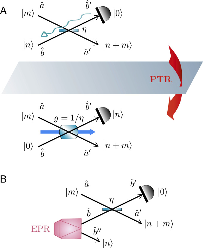
(A) PTR duality in a more general case with and photons impinging on modes and of a BS. By conditioning the output mode on vacuum and reversing the arrow of time, we get the same transition probability amplitude (up to a constant) as for a PDC of gain with input state and output state . (B) Corresponding operational scheme using an entangled (EPR) state at the input of mode . This makes it possible to access the output retrodicted state on mode .
The PTR duality is illustrated in Table 1 for few photons. As expressed by Eq. 7, it can be viewed as a consequence of partial transposition of the state of mode (leaving mode unchanged), namely the fundamental relation

| BS | PDC |
The second column (PDC) is obtained from the first column (BS) by timereversing mode , substituting with and dividing by the factor. The first row explains the latter factor: vacuum is obviously conserved in a BS, while PDC implies the stimulated emission of photon pairs (hence, the probability of keeping vacuum is strictly lower than one). The second and third rows correspond to the transmission of a single photon through the BS or PDC. The fourth and fifth rows correspond to the reflection of a single photon by the BS or the stimulated annihilation (fourth row) or emission (fifth row) of a photon pair by PDC.
(A) General statement of the PTR duality as expressed in Eq. 7, when and photons impinge on input modes and of a BS, while and photons are detected in output modes and . We recover a PDC with input and output . (B) Corresponding operational scheme, where a PDC is emulated with a BS. The input state of mode simply propagates through the BS and is projected onto . The input state of mode is converted, by projection on an EPR state, into the retrodicted state of mode , which back propagates through the BS and is projected onto in mode . We obtain the corresponding output state on mode by using an EPR pair. We thus recover a PDC with input and output , as encapsulated by Eq. 25.
We now prove PTR duality by reexpressing Eq. 24 in the Heisenberg picture, namely
Similar equations can be derived starting from and , which imply that the operator also commutes with and . Hence, is a scalar (proportional to ), and it is sufficient to compute its diagonal matrix element in an arbitrary state (e.g., ). Recalling that , we have , so that
Note that PTR duality can be reexpressed by using the identity
In the usual, predictive approach of quantum mechanics, one deals with the preparation of a quantum system followed by its time evolution and ultimately, its measurement. Specifically, one uses the prior knowledge on the state (prepared with probability ) in order to make predictions about the outcomes of a measurement . If the state evolves according to unitary before being measured, Born’s rule provides the conditional probabilities . In contrast, in the retrodictive approach of quantum mechanics (21), one postselects the instances where a particular measurement outcome was observed, and one focuses on the probability of the preparation variable conditionally on this measurement outcome. This can be interpreted as if the actually measured state had propagated backward in time to the preparer (Fig. 7A). Specifically, one associates a retrodicted state with the observed outcome and makes retrodictions about the preparation by evolving according to and applying a measurement , whose outcome discriminates the prepared state . In the simplest case (to which we restrict here) where there is no a priori information about the source, one sets . Then, by defining
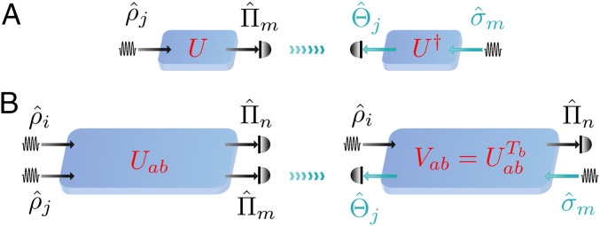
(A) Predictive (Left) and retrodictive (Right) pictures, describing the same experiment where state is prepared, evolves according to , and leads to measurement outcome associated with . The probability can be written as resulting from the retrodictive state back propagating according to , followed by measurement . (B) Predictive (Left) and intermediate (Right) pictures for a bipartite system. In the latter picture, associated with PTR, the retrodictive state of subsystem propagates backward in time, while the predictive state of subsystem propagates forward in time. If is a unitary, is not necessarily proportional to a unitary; however, it is the case when considering the BS vs. PDC duality.
The retrodictive picture can be successfully exploited in different situations [for example, to characterize the quantum properties of an optical measurement device (35)], but it is always used in lieu of the predictive picture. Here, we instead combine it with the predictive picture in order to properly define PTR duality and describe a composite system that is propagated partly forward and partly backward in time, as represented in Fig. 7 B, Right. Specifically, we consider a composite system prepared in a product state , then undergoing a unitary evolution followed by a product measurement . In the fully predictive picture (Fig. 7 B, Left), the conditional probabilities are given by
In our analysis of a BS under PTR, we have and , so that Eq. 33 reduces to Eq. 34. Hence, is unitary (up to a constant) and can be interpreted as the propagation of the retrodicted state of mode backward in time through the BS, while the predictive state of mode normally propagates forward in time through the BS. According to Eq. 40, the joint state is then shown to evolve according to a PDC. Note that it is not always possible to construct an operator that is proportional to a unitary operator, as it is the case here.
The HOM effect can be simply understood by calculating the probability amplitude for coincident detection
Now, we examine the corresponding quantum interferometric suppression in a PDC and its dependence in the parametric gain . Let us calculate the probability amplitude for coincident detection
We may also consider the case where the gain takes a larger integer value (e.g., ). A closer look at Eq. 46 reveals that the output term with photon pairs fully vanishes when is an integer. The corresponding distribution of the output photon pair number
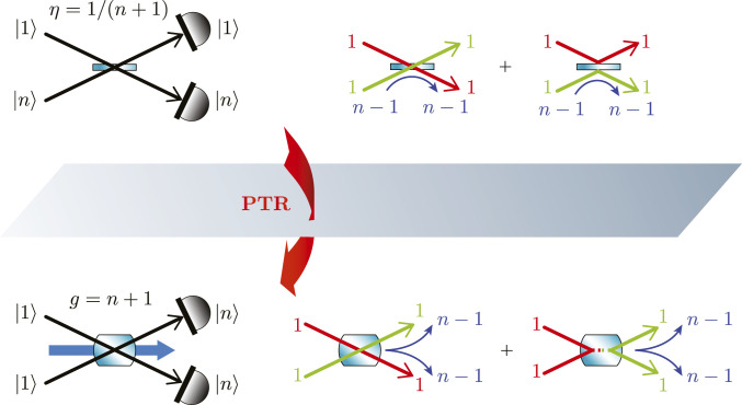
Extended quantum interferometric suppression in an amplifier where the detection of photon pairs at the output is suppressed if the gain . This is the PTR dual of the extended HOM effect when a single photon and photons impinge on the two input ports of an unbalanced BS of transmittance . The interference at play in the extended HOM is again the cancellation between a double reflection and double transmission (with other photons being always reflected from mode to mode ). Applying PTR, this translates into the cancellation between the amplitude for the two photons crossing the crystal and the amplitude for the stimulated annihilation combined with stimulated emission of the two photons (accompanied, in both cases, with the stimulated emission of pairs). In other words, the input pair may be up converted into the pump beam while pump photons are down converted, or the input pair may simply be transmitted while pump photons are down converted. Since the two scenarios are time-like indistinguishable, they interfere destructively.
The HOM effect is considered a most spectacular evidence of genuinely quantum two-boson interference, and we expect the same for its PTR counterpart as it admits no classical interpretation. The experimental verification of our effect can be envisioned with present technologies, as sketched in Fig. 9. We would need two single-photon sources, which could be heralded by the detection of a trigger photon at the output of a PDC with low gain (the single photon being prepared conditionally on the detection of the trigger photon in the twin beam). The two single photons would impinge on a PDC of gain 2, whose output modes should be monitored: the probability of detecting exactly one photon on each mode should be suppressed as a consequence of time-like indistinguishability. In principle, photon number resolution would be needed in order to discriminate the output term with one photon pair ( = 1) from the terms with more pairs ( 2). The ability of counting photons has become increasingly available over the last years (e.g., exploiting superconducting detectors), but this could also be achieved by splitting each of the two output modes into several modes followed by an array of on/off photodetectors. Experiments involving PDC in three coherently pumped crystals have already been achieved recently (36, 37), aiming at observing induced decoherence, so the proposed setup here should be implementable along the same lines. The squeezing needed to reach a gain 2 amounts to 7.66 dB, which is high but lies in the range of experimentally accessible values (in the continuous-wave regime). The experiment could alternatively be carried out with a lower gain (especially in the pulsed regime) provided the observed dip is sufficient to rule out a classical interpretation. As a matter of fact, a coincidence probability lower than 1/4 would be needed (see Classical Baseline), which could in principle be reached with a gain of 1.28 (i.e., a squeezing of 4.39 dB). Of course, the effect of losses should also be carefully analyzed in order to assess the feasibility of the scheme depicted in Fig. 9.
![Schematic of a potential demonstration of two-photon quantum interference in the amplification of light with gain 2. Two heralded single-photon sources (exploiting an avalanche photodetector [APD]) are used to feed the signal and idler modes of a PDC, and two photon number-resolving (PNR) detectors are used to monitor the presence of a single photon in each output port. The two-photon interference effect would be demonstrated by measuring a depletion of fourfold coincidences between the two trigger photons (heralding the preparation of two single photons) and the two output photons (here, the detectors should filter out the output states with ≥2 photons on each mode). The dominant terms will then consist of the stimulated annihilation of the two input photons (witnessed by two trigger photons but no output photons) as well as the stimulated emission of a photon pair (witnessed by two output photons but no trigger photons). When the time lapse between the detection of the trigger and output photons is close to zero (which means a perfect match of the timing of the output photons originating from the input photons associated with the trigger photons) the two terms should interfere destructively.](/dataresources/secured/content-1765760018179-aadf3d74-d338-4ace-9ff8-6de8b4593915/assets/pnas.2010827117fig09.jpg)
Schematic of a potential demonstration of two-photon quantum interference in the amplification of light with gain 2. Two heralded single-photon sources (exploiting an avalanche photodetector [APD]) are used to feed the signal and idler modes of a PDC, and two photon number-resolving (PNR) detectors are used to monitor the presence of a single photon in each output port. The two-photon interference effect would be demonstrated by measuring a depletion of fourfold coincidences between the two trigger photons (heralding the preparation of two single photons) and the two output photons (here, the detectors should filter out the output states with photons on each mode). The dominant terms will then consist of the stimulated annihilation of the two input photons (witnessed by two trigger photons but no output photons) as well as the stimulated emission of a photon pair (witnessed by two output photons but no trigger photons). When the time lapse between the detection of the trigger and output photons is close to zero (which means a perfect match of the timing of the output photons originating from the input photons associated with the trigger photons) the two terms should interfere destructively.
Demonstrating this effect would be invaluable in view of the fact that the HOM dip is widely used to test the indistinguishability of single photons and to benchmark mode matching: it witnesses the fact that the photons are truly indistinguishable (they admit the same polarization and couple to the same spatiotemporal mode). For example, HOM experiments have been used to test the indistinguishability of single photons emitted by a semiconductor quantum dot in a microcavity (10), while the interference of two single photons emitted by two independently trapped rubidium-87 atoms has been used as an evidence of their indistinguishability (15). The HOM effect has also been generalized to three-photon interference in a three-mode optical mixer (38), while the case of many photons in two modes has been analyzed in ref. 39, implying a possible application of the quantum Kravchuk–Fourier transform (40). We anticipate that most of these ideas could extend to interferences in an active optical medium.
The two-photon quantum interference effect in amplification cannot be interpreted within a classical model of PDC, where a pair can be annihilated or created with some probability. We have two possible indistinguishable paths (the photon pair either going through the crystal or being replaced by another one) with equal individual probabilities but opposite probability amplitudes; hence, the resulting probability vanishes (whereas the two probabilities would add for classical particles). In order to assess an experimental verification of this effect, it is necessary to establish a classical baseline, namely to determine the depletion of the probability of coincident detections that can be interpreted classically. As a guide, consider first a classical model of the HOM effect where the two input photons are distinguishable. We have to add the double-transmission probability with the double-reflection probability since these two paths can be distinguished. Then, the classical probability for coincident detections is
We thank Ulrik L. Andersen, Maria V. Chekhova, Claude Fabre, Virginia D’Auria, Linran Fan, Radim Filip, Saikat Guha, Dmitri Horoshko, Mikhail I. Kolobov, Julien Laurat, Klaus Mölmer, Romain Mueller, Ognyan Oreshkov, Olivier Pfister, Wolfgang P. Schleich, and Sébastien Tanzilli as well as an anonymous referee for useful comments. M.G.J. acknowledges support from the Wiener-Anspach Foundation. This work was supported by the Fonds de la Recherche Scientifique - FNRS under grant PDR T.0224.18.
There are no data underlying this work.
1
2
3
4
5
6
7
8
9
10
11
12
13
14
15
16
17
18
20
21
22
23
24
25
26
27
28
29
30
31
32
33
34
35
36
37
38
39
 Two-boson quantum interference in time
 Facebook
 Twitter
 Linkedin
 Whatsapp

