 A model and test for coordinated polygenic epistasis in complex traits
Proceedings of the National Academy of Sciences of the United States of America


Edited by Andrew G. Clark, Cornell University, Ithaca, NY, and approved December 2, 2020 (received for review February 19, 2020)
Author contributions: N.Z. and A.D. designed research; B.S., N.R., N.Z., and A.D. performed research; B.S., N.R., P.-R.L., and A.D. analyzed data; and B.S., N.R., P.-R.L., S.J.S., N.Z., and A.D. wrote the paper.
1B.S., N.R., N.Z., and A.D. contributed equally to this work.

- Altmetric
Systems-level interactions across physiological pathways, cell types, and tissues are core biological elements widely studied across diverse fields including evolution, systems biology, and model-organism genetics. However, they are essentially ignored in human genetics, and existing approaches fail to interpretably explain substantial complex trait heritability. Here, we propose the coordinated epistasis model of complex phenotypes that generalizes several recently proposed theoretical epistatic architectures of human traits. Broadly, coordination measures the degree to which epistasis effects act in concert with respect to marginal effects. It summarizes a dimension of polygenic effects orthogonal to parameters like heritability and standard estimates of epistasis.
Interactions between genetic variants—epistasis—is pervasive in model systems and can profoundly impact evolutionary adaption, population disease dynamics, genetic mapping, and precision medicine efforts. In this work, we develop a model for structured polygenic epistasis, called coordinated epistasis (CE), and prove that several recent theories of genetic architecture fall under the formal umbrella of CE. Unlike standard epistasis models that assume epistasis and main effects are independent, CE captures systematic correlations between epistasis and main effects that result from pathway-level epistasis, on balance skewing the penetrance of genetic effects. To test for the existence of CE, we propose the even-odd (EO) test and prove it is calibrated in a range of realistic biological models. Applying the EO test in the UK Biobank, we find evidence of CE in 18 of 26 traits spanning disease, anthropometric, and blood categories. Finally, we extend the EO test to tissue-specific enrichment and identify several plausible tissue–trait pairs. Overall, CE is a dimension of genetic architecture that can capture structured, systemic forms of epistasis in complex human traits.
Interaction between the phenotypic effects of genetic variants, or epistasis, is an essential component of biology with important consequences across multiple scientific domains. For example, epistasis significantly impacts evolutionary models, including response to selection or changing environment (1, 2). Epistasis also fundamentally shapes genetic architecture, as the direction of an allele’s effect can change based on genetic background (345–6). Epistatic interactions are pervasive in model systems, including in model organisms (2, 78910–11) and in recent mammalian gene-level interaction screens (121314–15). Moreover, these interactions often represent core biological functions. For example, the molecular chaperone HSP90 modifies diverse disease-model–specific proteins (1617–18), and conceptually similar mechanisms protect the cell from aberrant translation at ribosomes (19). Such highly structured forms of epistasis are a core focus of systems biology, and their genetic bases have long been hypothesized to influence complex human disease.
While the observations in model organisms suggest that epistasis is also fundamental in humans (11, 20), it remains poorly understood. This is largely because powerful, interpretable modeling tools are nascent. Genome-wide searches for interacting single-nucleotide polymorphism (SNP) pairs are computationally and statistically onerous, despite some success (21). Additionally, recent and classical methods for epistasis increase power by aggregating interactions across the whole genome (3, 222324252627–28), and their results further support the potential importance of epistasis in complex traits. Interestingly, all of these approaches assume that interaction effect sizes and directions are independent of main effects or, in other words, that epistasis is uncoordinated.
This is in contrast with recent conceptual models of complex human traits that imply or are consistent with coordinated forms of epistasis. For example, Zuk et al. describe a limiting pathway model of human disease that directly implies negative interactions between SNPs contributing to different pathways (29). Also, the HSP90 community has discussed the possibility of a polygenic version of chaperon function (30), which would induce coordinated interactions between HSP90 buffer SNPs and exonic missense SNPs. Another example is the omnigenic model, which suggests that traits are determined by a few trait-specific “core” genes that are modified by many nonspecific “peripheral” genes (31, 32), implying coordinated epistasis (CE) between the SNPs contributing to “core” and “peripheral” genes. Monogenic disorders with polygenic modifiers are another instance of structured epistasis, where the expressivity and penetrance of mutations in a core gene are modified by many variants distributed among the genome (3334–35).
Motivated by these concerns, we formally propose a concrete parameter to capture a specific form of structured epistasis, which we call CE and define formally below. Conceptually, CE measures concerted interactions between pathways that are themselves additively heritable traits. For example, one pathway might capture additive genetic effects on a polygenic buffering pathway, similar to HSP90, and another pathway might capture genetic effects on individual proteins that contribute to disease. In another example, type 2 diabetes (T2D) involves interactions between insulin-sensing and -producing systems, which likely have distinct genetic architectures and operate through different tissues (3637–38). We quantify CE with the parameter , where indicates negative epistasis between genetic pathways, on average, dampening the marginal effects of trait-increasing variants; conversely, indicates positive epistasis, where trait-increasing SNP effects are actually magnified in the full organismal context relative to their genome-wide association study (GWAS) estimates. Importantly, CE is a test for general statistical epistasis and does not generally indicate the present of biological interactions as in a protein complex (35).
For simplicity, we usually imagine CE in the context of positive SNP effects, where positive/negative epistasis coincide with the more interpretable notions of synergy/antagonism. For example, for a disease trait, positive epistasis and synergy both imply that the joint effect of risk alleles exceeds the sum of their marginal effects. In general, however, CE measures the skew in genetic risks, and may either dampen or exacerbate marginal genetic effects (39). In Fig. 1, we illustrate in the case of two latent interacting risk pathways. The key is that if there are heritable, positively (synergistically) or negatively (antagonistically) interacting pathways (Fig. 1B), while if the interactions are purely random or if the interactions are absent (Fig. 1A).

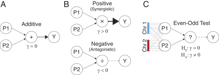
CE and the EO test with two chromosomes. (A) In the additive model, SNP effects from the two phenotype-increasing pathways are summed to produce the phenotype . (B) Same as A, except the pathways interact either positively (synergistically, ) or negatively (antagonistically, ). (C) The EO test considers interaction from traits derived from the even and odd chromosomes in place of the unknown pathways truly driving the interaction.
Testing for the existence of CE would be straightforward if we knew or could accurately estimate the SNP effects on causal, latent pathways: we could simply build genetic predictors of each pathway and test their interaction. However, these pathways are generally unknown and high dimensional, making CE estimation seem impossible. Surprisingly, we prove that testing for CE can be accomplished by randomly assigning independent sets of SNPs to arbitrary proxy pathways. Concretely, we build polygenic risk scores (PRS) specifically for the even and odd chromosomes and then test their interaction in a linear regression on phenotype (Fig. 1C). We call this the even–odd (EO) test, and we prove analytically that EO reliably estimates CE under polygenicity. We also prove that under a polygenic model, any chromosome split, not just EO, gives identical results in expectation. Importantly, however, partitions aligned closely with the true latent pathways will have greater power. We leverage this fact to test for CE enrichment in specific genomic annotations. Specifically, we focus on tissue-specific annotations to ask whether complex traits are enriched for interactions between tissue-specific pathways.
In this paper, we first introduce the concept of CE formally and define the EO test. We then examine simulated data sets to show that EO is robust to confounding under plausible models of assortative mating and population structure. Then, we perform the EO test in the UK Biobank (UKBB) across 26 traits spanning multiple domains and find 18 with significant CE. We validate the approach, which uses internally cross-validated PRS, by using PRS constructed from external data sources for 17 of the 26 traits. Finally, we estimate tissue-specific CE across 13 tissues in the UKBB and find several biologically plausible tissue–trait pairs, including several that replicate, as well as enrichment for interacting tissue pairs. We conclude with a discussion of limitations to our approach, implications for association testing and genetic architecture, and possible future extensions.
Results
Coordinated Polygenic Epistasis.
Throughout the paper, we assume a polygenic pairwise epistasis model:
The standard additive model assumes no epistasis, that is, . In this model, SNP always has the same effect on the phenotype, regardless of genetic background or environment. In the polygenic setting, where there are many more SNPs than individuals (M > N), total heritability can still be reliably estimated by the random-effect model Genome-based restricted maximum likelihood (GREML), which models as i.i.d. Gaussian (40).
Epistatic models go further by allowing nonzero . To date, epistatic tests have focused either on candidate SNPs or genome-wide screens for SNP pairs, which reduce M < N and facilitate simple fixed-effect models (21). More recently, random-effect models akin to GREML have become popular for estimating the total size of (i.e., the heritability from pairwise epistasis) (252627–28). Another recent approach tests for interaction between a single SNP and a genome-wide kinship matrix, a useful compromise that provides SNP-level resolution and also aggregates genome-wide signal (22).
While these methods are useful for characterizing the existence and impact of epistasis, all are limited by the assumption that and are independent. We are interested in an orthogonal question: when are and deeply intertwined by latent interacting pathways? Conceptually, and encode all relevant information, so the goal is to decode the presence of interacting pathways from these parameters. Concretely, we prove that these pathways exist if, and only if, the CE is nonzero, where is defined as:
As a stylistic example, imagine there are two genetically independent pathways that are each sufficient for T2D, one based on body mass index (BMI) and one based on pancreas function. Then is expected, because high-BMI cases are not likely to also have high pancreas risk, which is rare. On the other hand, if a disease requires high risk across distinct systems, then is expected. As another stylistic example, if asthma requires both immune components and tobacco exposures, then the impact of a smoking-risk SNP on asthma is greater in the presence of immune risk factors.
We provide a more rigorous exploration of coordination in SI Appendix. In particular, we prove that several biologically plausible epistasis models induce CE, including a trans genetic regulation model (32) (SI Appendix, section 4.1), a polygenic generalization of molecular buffers (16) (SI Appendix, section 4.2), and gene–environment interaction with heritable environment (41) (SI Appendix, section 4.3 and Fig. S1). We also show that within-pathway coordination contributes to CE and can cause (SI Appendix, Example 3 and Fig. S2). We also study CE as a function of the number of latent pathways; in particular, results in the mathematically natural many-pathway limit, hence CE typically indicates the existence of a parsimonious set of interacting pathways (SI Appendix, Example 4).
The EO Estimator for CE.
We have defined our target, the CE , as a function of the true genetic effects and However, these parameters are not known; even worse, they are high dimensional and cannot be accurately estimated. Nonetheless, we develop a simple and powerful method to test for nonzero .
The key idea in the EO test is that randomly defined pathways can act as proxies for true pathways. These random pathways will have a significant interaction if, and only if, there truly are latent pathways that interact. Intuitively, this randomized approach has power to detect true signals because many interacting SNP pairs are appropriately assigned under the random partition—the probability of incorrectly assigning all interacting pairs is negligible. Furthermore, the EO test is calibrated because incorrectly assigned SNP pairs do not interact and hence do not cause bias. In other words, correctly assigned SNP pairs will exist and will suffice to drive interactions between the even and odd proxy pathways. Although the incorrectly assigned SNPs will cause power loss and downward bias for , this bias can be corrected post hoc if we assume an infinitesimal epistatic model (SI Appendix, Proposition 1). In this case, exactly half of all interacting SNP pairs will be captured by the random SNP partition, which allows us to perfectly estimate the aggregate contribution of SNPs whose pairwise interactions are not captured by the EO partition. Mathematically, these facts are related to other randomized approaches for high-dimensional estimation, including GREML, randomized linear algebra, and compressed sensing (42434445–46).
We propose estimating by regressing on the interaction between PRS built specifically from even-indexed and odd-indexed chromosomes ( and , respectively):
Our choice of even and odd chromosomes is clearly arbitrary. Crucially, we prove that any partition of chromosomes into two groups without linkage disequilibrium (LD) gives identical results under a perfectly infinitesimal model (SI Appendix, section 3.2). Therefore, for concreteness, simplicity, and to emphasize the arbitrariness and flexibility of the EO test, we have chosen to define it by the case where one PRS is built specifically from SNPs on even chromosomes and the other is built specifically from SNPs on odd chromosomes.
With finite genomes, however, results may depend heavily on the precise choice of chromosomes used to build and . Nonetheless, it is important that SNPs are independent across splits to avoid false positives from nonlinear single-variant effects, that is, dominant or recessive variants. Hence, we always evaluate chromosome-level genome partitions. This is analogous to our choice to exclude the terms from CE; in both cases, CE implies nonlinear effects of each individual SNP and the aggregate PRS, but the converse is not true. In practice, we use a more flexible form for the EO test, where we jointly fit and test the interactions between all (22 choose 2) chromosome-specific PRS, which simultaneously obviates LD concerns and the arbitrariness of assigning chromosomes based on their canonical indices. Nonetheless, our method does not assume the true causal pathways are located in contiguous or independent genomic regions; rather, this is a condition on our chosen partition of the genome that is used in the EO test. In particular, both CE and EO remain valid when causal SNPs for each pathway are distributed across the genome randomly, and/or when SNPs contribute to multiple pathways (SI Appendix, section 3.3).
EO Test Can Distinguish CE from Population Structure and Uncoordinated Epistasis.
To examine the properties of the EO test, we simulate data under three biologically plausible genetic architectures: additivity, isotropic (i.e., uncoordinated) epistasis, and CE. For each architecture, we also test the impact of population structure, assortative mating, and adjustment with principal components (see Materials and Methods). In each case, we perform a GWAS and then build ordinary PRS as well as PRS based only on variants from odd chromosomes and even chromosomes ( and respectively). We then test PRS in a second dataset.
We first tested the correlation between and , called , which is related to an existing method of assortative mating (47). We found that the test for reliably indicated the presence of assortative mating or uncorrected population structure. Note that after adjusting for PCs, the test for was roughly null in the presence of population structure (Table 1).

| Simulation characteristics | |||||||
| Population structure | PC adjusted | Assortative mating | PR (α = 0.05) | PR (α = 0.05) | |||
| Additive | N | N | N | 1.0 (1.4) | 0.05 | 1.0 (1.4) | 0.05 |
| Y | N | N | 81,789.4 (35,386.7) | 0.99 | 101.1 (50.5) | 0.95 | |
| Y | Y | N | 1 (1.4) | 0.05 | 1.0 (1.4) | 0.05 | |
| N | N | Y | 40.7 (13.0) | 1.00 | 1.1 (1.6) | 0.06 | |
| Isotropic epistasis | N | N | N | 1.0 (1.4) | 0.05 | 1.0 (1.4) | 0.05 |
| Y | N | N | 81,698.3 (35,422.0) | 0.99 | 101.0 (51.1) | 0.95 | |
| Y | Y | N | 1.0 (1.4) | 0.05 | 1.0 (1.4) | 0.05 | |
| N | N | Y | 40.6 (12.9) | 1.00 | 1.2 (1.7) | 0.08 | |
| CE | N | N | N | 1 (1.4) | 0.05 | 15.4 (8.3) | 0.96 |
| Y | N | N | 81,717.4 (35,394.7) | 0.99 | 109.6 (57.1) | 0.96 | |
| Y | Y | N | 1.0 (1.4) | 0.05 | 14.2 (8.2) | 0.93 | |
| N | N | Y | 40.8 (12.9) | 1.00 | 43.4 (14.9) | 1.00 | |
| Oracle EO partition | N | N | N | 1.0 (1.4) | 0.05 | 132.6 (25.2) | 1.00 |
Mean, standard deviation (SD), and positive rate (PR) at nominal P < 0.05 are shown for estimates of and . We display results averaged over 10,000 simulations using the baseline parameters n = 10,000, h2 = 0.5, and γ = 0.2. For all models, the ordinary EO test was performed by randomly assigning SNPs to either the “Even” or “Odd” group, except in the “Oracle EO Partition” setting where SNPs were grouped according to the true, generative pathways they causally effect.
However, our main focus is on the EO test for . We found that the EO test was calibrated under both the additive and isotropic interaction models, as expected, with false-positive rates near 0.05 at a nominal P < 0.05 threshold. In particular, this is a clear demonstration of a setting where significant pairwise epistasis exists and yet CE does not exist, thereby drawing a clear distinction between CE and the more general concept of epistasis. Further, the EO test has power of roughly 95% under the CE model (Table 1).
We did not observe substantial false positives in the EO test under assortative mating. However, we did observe high false-positive rates for the EO test under uncorrected population structure (0.95), although after correcting for PCs, the test is calibrated with an empirical false-positive rate near 0.05 (Table 1). In practice, we recommend adjusting for population-structure proxies when running the EO test, as is standard in human genetics.
We then sought to more comprehensively profile the behavior of the EO test across a range of simulation parameters. First, we varied the sample size, n (SI Appendix, Fig. S3A). As expected, power at nominal P < 0.05 grew with sample size, from roughly 5% at n = 1,000, up to roughly 95% at n = 10,000 (our baseline), and reaching nearly 100% at n = 20,000. Next, we varied the additive heritability, which affects the EO test power because it governs the accuracy of the PRS estimates (SI Appendix, Fig. S3B). As expected, power increased with heritability, growing from 35% at h2 = 0.1 to nearly 100% at h2 = 0.7 (our baseline is h2 = 0.5). Finally, we varied the strength of CE parameter, . As expected, power grew with , reaching 100% when we doubled the parameter relative to our baseline (SI Appendix, Fig. S3C). Furthermore, when , we recovered calibrated tests with roughly 5% false-positive rate. Interestingly, our simulations had similar power regardless the sign of , as expected because the sign of the phenotype is arbitrary in these simulations.
An essential feature of the EO test is that it is unbiased even when the even/odd partition of SNPs is chosen randomly with respect to partition of SNPs into the causal interacting pathways (under conditions stated above). Nonetheless, the power to detect CE increases when the even/odd partition more closely aligns with the causal partition; we demonstrate this in our simulations by directly matching the two partitions (see Materials and Methods). As expected, the EO test power increases from 95 to 100% when we use this more precise SNP partition (Table 1).
Our above simulations used minor allele frequencies (MAFs) drawn i.i.d. from a uniform (0.01,0.5) distribution. To assess a more realistic MAF spectrum, we repeated our baseline simulations using MAFs drawn randomly from the MAF spectrum we observed in UKBB, excluding rare variants with MAF < 0.01 for simplicity. Nonetheless, the simulation results were nearly identical (SI Appendix, Table S1).
Finally, we assessed the EO test under third-order epistasis (SI Appendix, Table S2). First, when interacting SNP triples were distributed uniformly at random across the genome, as in the isotropic model of pairwise epistasis, the EO test had positive rate near 0.05. This is appropriately calibrated behavior in the informal sense that there is no relationship between main effects and epistasis effects and in the formal sense of the definition of CE (Eq. 1, above). Second, we simulated a three-pathway model where the product of all three pathways, but not any two, had an effect on the phenotype. In this setting, the main and interaction effects are related, but the formal CE definition is still 0. In the simulation, we observe power near 8% at P < 0.05 significance. This is expected in our simulations that use finite genomes; for any simulated dataset, the pathways will have some nonzero mean that induces pairwise interaction, resulting in an average estimate that is zero but overdispersed (this is related to similar issues in GREML with finite numbers of causal SNPs) (48). Overall, the EO test is calibrated under isotropic third-order epistasis and has some signal under higher-order coordinated epistasis.
Testing for CE with the EO Test in the UKBB.
We next tested for CE with the EO test in the UKBB (49). We studied 21 quantitative and 5 binary traits (SI Appendix, Table S3) chosen to represent a range of trait classes including anthropometric, disease, and blood traits. We specifically analyzed the subjects classified as “White British” and filtered out related individuals to minimize population structure bias while retaining large sample sizes (max n = 342,816). We calculated PRS for each chromosome for each sample using a standard thresholding approach (50) (see Materials and Methods). The total PRS is then the sum of the individual chromosomes’ PRS. We evaluated a range of PRS P value thresholds and corrected for this source of multiple testing using a Benjamini–Hochberg false discovery rate (FDR) threshold of 10%. We used 10-fold cross-validation across individuals to minimize bias from in-sample overfitting.
Unlike in perfectly infinitesimal models, in real data, the EO test depends on the specific partition of chromosomes used to estimate . To minimize bias from choosing a single split, for example, even versus odd, in practice we jointly test interactions across all distinct pairs of chromosome-specific PRS with an F-test (see Materials and Methods). Following common practice (5152535455–56), we report the significant results per phenotype.
We discovered 18 traits with significant CE (Table 2), including the complex diseases asthma, cardiovascular disease (CVD), eczema, and T2D. We also detected CE for the complex quantitative traits basal metabolic rate, bone mineral density (BMD), lung function (forced expiratory volume [FEV]/ forced vital capacity [FVC]), and height, as well as nine blood traits: glucose, low density lipoprotein (LDL), platelet distribution width, mean platelet volume (MPV), red blood cell distribution width, sphered cell volume, triglycerides (TG), and counts of monocytes, lymphocytes, and platelets (PLAT). Taken together, these results show that CE contributes to the genetic architecture of multiple complex traits.
| Phenotype | PRS type | τ | %VE | FDR |
| Basal metabolic rate | Intern quant | 1.00E-08 | 0.74 | 0.02 |
| BMD | Intern quant | 0.001 | 3.39 | 2.30E-03 |
| FEV/FVC | Intern quant | 1.00E-07 | 0.52 | 0.02 |
| Glucose | Intern quant | 1.00E-05 | 2.28 | 0.02 |
| Height | Intern quant | 1.00E-08 | 2.80 | 4.00E-03 |
| LDL | Intern quant | 1.00E-07 | 1.30 | 7.30E-04 |
| Lymphocyte no. | Intern quant | 1.00E-05 | 1.05 | 2.00E-03 |
| Monocyte no. | Intern quant | 1.00E-08 | 0.95 | 8.60E-04 |
| PLAT no. | Intern quant | 0.0001 | 5.81 | 0.08 |
| PLAT distribution width | Intern quant | 1.00E-08 | 3.99 | 2.60E-04 |
| PLAT volume | Intern quant | 0.0001 | 9.06 | 2.90E-11 |
| RBC distribution width | Intern quant | 1.00E-06 | 2.04 | 0.01 |
| Sphered cell volume | Intern quant | 1.00E-06 | 1.73 | 0.07 |
| Triglycerides | Intern quant | 0.0001 | 1.55 | 9.70E-03 |
| Asthma | Intern bin | 0.0001 | 2.79 | 6.60E-04 |
| Cardiovascular | Intern bin | 1.00E-08 | 3.90 | 6.50E-05 |
| Eczema | Intern bin | 1.00E-08 | 2.18 | 8.10E-05 |
| T2D | Intern bin | 0.001 | 3.64 | 9.40E-08 |
| Corp. hemoglobin | Extern quant | — | 19.17 | 0.04 |
| LDL | Extern quant | 1.00E-05 | 2.19 | 0.01 |
| PLAT no. | Extern quant | — | 16.90 | 5.20E-03 |
| PLAT volume | Extern quant | — | 29.41 | 1.10E-25 |
Significant traits based on either internal or external PRS are shown (FDR < 0.1); results for all traits are shown in SI Appendix, Table S3. We summarize evidence for CE per trait using Benjamini–Hochberg FDR across nine PRS P-value thresholds; for single-threshold external PRS, FDR is just an ordinary P value. “Intern” indicates that the PRS was calculated using the cross-validation method with UKBB data (Materials and Methods). “Extern” indicates that the PRS was calculated using GWAS summary statistics from external datasets (Materials and Methods). is the marginal SNP P-value threshold used to construct the PRS and that minimizes the EO test P value. %VE describes the variance explained by the chosen PRS across all samples. quant, quantitative.
To assess the potential for impact by population structure and assortative mating, we calculate the correlation between each pair of chromosome-specific PRS . In simulations, we found that indicates the presence of structured genotypes, which may be due to assortative mating and/or uncorrected population stratification. Although correction for PCs was sufficient for calibrated inference in simulations (Table 1), we nonetheless studied the relationship between and as a metric for possible confounding of the EO test by stratification. This caution is motivated by the complexities of population structure in massive datasets like the UKBB (575859–60). However, we found no evidence that population stratification drove our CE inference; larger values of did not correlate with values or their corresponding P or log(P) values (SI Appendix, Fig. S4). Overall, even with these conservative extra tests we did not identify evidence that our EO test for CE was substantially confounded by uncorrected structure or assortative mating.
As a final assessment, we repeated our EO test for 100 random permutations of the PRS among samples. The resulting EO-test FDR was null, as expected (SI Appendix, Fig. S5). Furthermore, we used these permutations to construct empirical P values for the minimum EO test across all PRS thresholds as an alternative to FDR correction. This gives qualitatively similar results to our primary FDR-based analysis, although computational costs bound the minimum attainable empirical P values (SI Appendix, Fig. S6). These analyses do not rule out the possibility of subtle confounding, but they do provide further support for the calibration of the EO test in practice.
Replicating EO Test Results with External PRS.
Although we have cross-validated our PRS, we wished to additionally check that our results are not specific to a single population by overfitting dataset-specific confounders (57, 58, 60). We investigated this by constructing PRS using external summary statistics to remove the potential impact of cohort-specific artifacts. We selected eight traits that have large external GWAS summary statistics: asthma, T2D, CVD, height, BMI, TG, educational attainment, and LDL; additionally, we constructed PRS for nine other blood traits that were only available for a specific P-value threshold (see Materials and Methods and SI Appendix, Table S3). We tested replication for the 10 traits in this list with internally significant CE.
We applied the EO test as described above and found that CE replicated for LDL, PLAT, and MPV (Table 2). This validates CE in the sense that our results are not specific to the main effect–size estimates derived from the UKBB dataset. However, significant CE did not replicate for several traits. Broadly, the CE P values were less significant using external PRS, likely due to a combination of winner’s curse and the fact that external studies generally analyze datasets smaller than UKBB and do not perfectly match UKBB in terms of environment and genetic background.
To further strengthen confidence in CE, we performed an alternate replication analysis by directly comparing the internal and external PRS-interaction effect estimates across all pairs of chromosomes (Fig. 2). This test identified highly significant CE replication for 7/10 tested traits. This test is more powerful than simply applying the EO test to the external PRS because it tests a narrower alternative hypothesis. Specifically, the EO test asks whether any chromosome pairs interact, whereas the direct replication test asks whether the external interaction effect estimates correlate with their internal counterparts. Conceptually, this is related to one- versus two-sided tests, as the former add power when prior knowledge of the estimand’s sign is available.
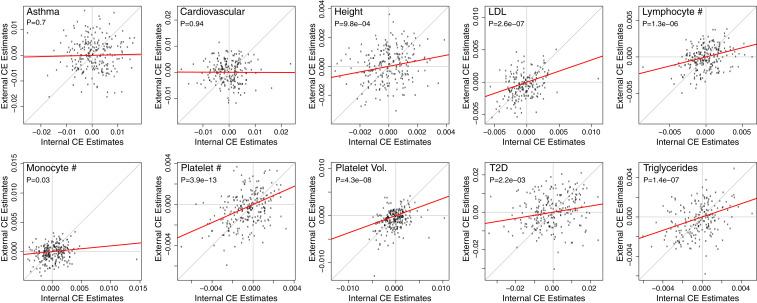
CE replication in UKBB. For each of the 10 phenotypes with internally significant CE and with available external PRS, we plot internal interaction estimates (x-axis) against external estimates (y-axis) for each pair of chromosomes. Chromosomes that do not contribute to a particular PRS are excluded. We use the PRS P-value threshold for each PRS to minimize its CE P value; this does not cause inflation because we are not testing the size of these interaction estimates but rather their correlation. This indirect replication test is Bonferroni significant for 7/10 traits when correcting for the number of tested traits. Effect sizes are displayed after each chromosome-specific PRS is centered and scaled, and the P values and red lines correspond to regressions with intercepts constrained to 0.
In addition to strengthening confidence in the existence of CE, these replication analyses also suggest that CE can be reliably tested using internally constructed PRS in the future. This can be essential for applications to under-studied traits, populations, or environmental contexts (61626364–65).
Tissue-Specific Coordination in UKBB.
Having demonstrated the existence of CE for several traits, we now consider the possibility that interacting pathways are enriched in trait-relevant tissues. Specifically, we test for tissue-specific enrichment of CE across the above 26 traits and 13 tissue-specific genomic annotations: 7 based on specifically expressed genes (adipocytes, blood cells, brain, hippocampus, liver, muscles, and pancreas) (66, 67) and 6 based on tissue-specific chromatin-marker patterns (adipose, brain, hippocampus, liver, pancreas, and skeletal muscle) (68, 69) as used in ref. 51.
For each tissue–trait pair, the tissue-specific EO test asks whether the coordination mediated through a specific tissue exceeds the genome-wide average. This test is conducted by first creating a tissue-specific PRS for each chromosome and testing it for interaction with the standard PRS on other chromosomes (, ). To focus our test on truly tissue-specific effects, rather than global effects that happen to be tagged by tissue-specific regions, we adjust for the ordinary chromosome-level PRS interactions as well as the main effects of each chromosome’s PRS and TPRS. We use a P = 0.05 threshold with a conservative Bonferroni correction to account for the multiple tested tissues. We only evaluate phenotypes with significant ordinary CE (Table 2).
We found 53 instances of tissue-specific CE enrichment using internal PRS (Table 3 and SI Appendix, Table S4). This includes nine tissues enriched for LDL CE, several of which are essentially positive controls: the liver is a key regulator of LDL metabolism and adipocytes and muscles are primary sinks for the triglycerides carried by LDL (70). Further confirming these results, adipocyte CE-enrichment replicates when using external LDL PRS.
| Phenotype | Tissue | PRS type | TPRS %VE | P value |
| BMD | Liver | Intern quant | 1.07 | 1.80E-03 |
| FEV/FVC | FrankelLiver | Intern quant | 0.28 | 1.30E-06 |
| Glucose | Franke.muscles | Intern quant | 0.07 | 2.40E-04 |
| Height | Franke.blood.cells | Intern quant | 0.03 | 4.00E-12 |
| LDL | Franke.blood.cells | Intern quant | 0.10 | 1.10E-04 |
| LDL | Franke.adipocytes | Intern quant | 1.77 | 2.60E-04 |
| LDL | Franke.brain | Intern quant | 1.10 | 6.60E-04 |
| LDL | Franke.hippocampus | Intern quant | 0.38 | 6.50E-06 |
| LDL | Franke.liver | Intern quant | 3.02 | 1.60E-03 |
| LDL | Franke.muscles | Intern quant | 0.26 | 1.30E-03 |
| LDL | Franke.pancreas | Intern quant | 1.95 | 2.00E-03 |
| LDL | Brain | Intern quant | 4.71 | 2.90E-04 |
| LDL | Hippocampus | Intern quant | 4.24 | 1.60E-05 |
| Lymphocyte no. | Franke.hippocampus | Intern quant | 0.90 | 2.10E-03 |
| Monocyte no. | Franke.hippocampus | Intern quant | 0.15 | 4.30E-04 |
| PLAT no. | Franke.adipocytes | Intern quant | 1.03 | 1.10E-03 |
| PLAT no. | Franke.hippocampus | Intern quant | 0.39 | 7.60E-05 |
| PLAT no. | Franke.muscles | Intern quant | 0.17 | 1.20E-03 |
| PLAT no. | Skeletal_muscle | Intern quant | 2.92 | 1.80E-03 |
| PLAT distribution width | Franke.brain | Intern quant | 0.04 | 5.30E-04 |
| PLAT volume | Franke.blood.cells | Intern quant | 0.36 | 1.80E-04 |
| PLAT volume | Franke.adipocytes | Intern quant | 1.83 | 9.60E-07 |
| PLAT volume | Franke.brain | Intern quant | 0.00 | 1.40E-09 |
| PLAT volume | Franke.hippocampus | Intern quant | 0.02 | 6.80E-13 |
| PLAT volume | Franke.liver | Intern quant | 1.27 | 1.30E-03 |
| PLAT volume | Franke.pancreas | Intern quant | 0.62 | 1.30E-04 |
| PLAT volume | Skeletal_muscle | Intern quant | 0.62 | 3.60E-03 |
| Sphered cell volume | Franke.blood.cells | Intern quant | 0.51 | 3.00E-03 |
| Triglycerides | Franke.pancreas | Intern quant | 0.49 | 6.60E-04 |
| Cardiovascular | Franke.brain | Intern bin | 0.01 | 8.20E-05 |
| Cardiovascular | Franke.liver | Intern bin | 0.24 | 1.00E-04 |
| Cardiovascular | Franke.muscles | Intern bin | 0.04 | 2.10E-04 |
| Cardiovascular | Adipose | Intern bin | 0.26 | 1.70E-03 |
| Eczema | Franke.muscles | Intern bin | 0.07 | 2.10E-04 |
| LDL | Franke.adipocytes | Extern quant | 0.44 | 2.30E-03 |
| PLAT volume | Franke.adipocytes | Extern quant | 0.08 | 1.60E-08 |
| PLAT volume | Franke.brain | Extern quant | 0.02 | 2.90E-03 |
| PLAT volume | Franke.muscles | Extern quant | 0.06 | 4.70E-05 |
| PLAT volume | Franke.pancreas | Extern quant | 0.00 | 7.40E-05 |
| PLAT volume | Adipose | Extern quant | 0.13 | 1.10E-03 |
| PLAT volume | Brain | Extern quant | 0.02 | 3.30E-03 |
| PLAT volume | Liver | Extern quant | 0.00 | 4.60E-04 |
Trait–tissue pairs with significant tissue-specific CE are shown; results for all tested trait–tissue pairs are in SI Appendix, Table S4. For parsimony, we list here only the most significant tissue per trait as well as all significant tissues for traits discussed in the main text. The prefix “Franke.” indicates that the tissue annotation is derived from Franke laboratory (66, 67). TPRS %VE is percent phenotype variance explained by the tissue-specific PRS. P values for the tissue-specific CE estimate are Bonferroni adjusted for testing across multiple tissue annotations. “Intern” indicates that the PRS was calculated using the cross-validation method with UKBB data (Materials and Methods). “Extern” indicates that the PRS was calculated using GWAS summary statistics from external datasets (Materials and Methods).
Another biologically plausible set of tissue–trait pairs is for MPV, which also had the strongest ordinary CE of any trait. First, we find significant enrichment for liver, consistent with its known role as the main producer of the main regulator of PLAT production, thrombopoietin (TPO) (71). Second, we find significant CE enrichment for muscles, which also modestly produce TPO (71); furthermore, PLATs are important in healing muscles. Third, we found suggestive CE with brain tissues—while the underlying biology is less obvious, there is evidence that TPO affects brain development (72). Additionally, recent complementary studies have found evidence that brain tissue plays a role in MPV (73). All three of these tissues replicate for CE enrichment when using external PRS.
We also found tissue-specific CE for complex disease. For example, CVD has CE enrichment for brain, liver, muscle, and adipose and has a clear link to CVD; several brain regions have been implicated in the genetic basis of BMI, a CVD risk factor (74, 75), and liver, muscle, and adipose all are deeply involved in energy homeostasis (76). While none of these tissues replicate, this likely reflects lack of power as even ordinary CE was not significant in either of our external replication tests.
To add further confidence in tissue-specific CE, we tested five permutations of the TPRS across samples. We observed that the resulting P values were appropriately null (SI Appendix, Fig. S7).
In general, the tissue-specific EO test can improve power over the ordinary EO test when the correct tissue is identified, despite the fact that the TPRS almost necessarily explain less trait variation than the overall PRS. This is consistent with our simulation result where the EO test power increased under the Oracle approach that partitions SNPs into the true pathways, even though this yields PRS with weaker predictive power. For example, the empirical EO test P value for sphered cell volume is 0.03 (SI Appendix, Table S3), but its P value for blood-cell CE is 0.003; however, the overall PRS explains 1.5% of trait variance while the blood-cell TPRS explains only 0.5%. Similar properties can be observed for many plausible tissue–trait pairs, for example, in the liver-specific CE for glucose and triglycerides. This is further evidence that CE is truly enriched in specific tissues for some traits and illustrates that CE captures a genetic axis that is partially distinct from additive variance.
Tissue-Pair CE in UKBB.
We next ask whether CE can be detected between pairs of tissues based on the hypothesis that pathways may be tissue specific. Rather than test the interaction between tissue-specific PRSi and global PRSj, we now test for interaction between tissue 1–specific PRSi and tissue 2–specific PRSj. For tissue-specific CE, we adjust for the same covariates as above and now additionally adjust for for both tested TPRS and all . In particular, these tissue–tissue interaction tests are statistically independent of the EO tests and the tissue-specific tests in the above sections under the null hypothesis for tissue–tissue interaction.
If tissue–tissue CE exists, it will likely cause tissue-specific CE; hence, to improve power, we only test tissue–trait pairs that are significant in the above TPRS test (internal or external, Table 3). This reduction in testing dimension is particularly important here because the number of tests scales by the number of evaluated tissues squared. As each phenotype now has a different number of tests, and this test is the most complex and high dimensional we consider, we use an aggressive Bonferroni correction and adjust for all tested trait-tissue-tissue triples, performed separately for internal and external PRS.
We find five Bonferroni-significant examples of tissue–tissue CE (Table 4 and SI Appendix, Table S5). Two highlight the role of muscles in PLAT, one interacting with adipocytes (internal is significant; external P = 0.02), and another with hippocampus (external is significant; internal P = 0.01); despite the nominal internal/external replication, the biological interpretation of these tissue pairs is unclear. Two other tissue pairs highlight brain interaction with blood cells and liver for MPV; again, the role of the brain is not clear, but both blood cells and liver have strong connection to MPV biology. Finally, we find evidence for liver–pancreas CE driving FEV/FVC1, which is particularly striking as the P value for this tissue–tissue CE exceeds either P value for these tissues’ individual CE.
| Phenotype | Tissue 1 | Tissue 2 | PRS type | P value |
| FEV/FVC | Franke.liver | Franke.pancreas | Intern quant | 2.20E-05 |
| PLAT no. | Franke.adipocytes | Franke.muscles | Intern quant | 1.50E-04 |
| PLAT volume | Franke.blood.cells | Franke.brain | Intern quant | 1.80E-05 |
| PLAT volume | Franke.hippocampus | Franke.liver | Intern quant | 2.30E-04 |
| PLAT no. | Franke.hippocampus | Franke.muscles | Extern quant | 2.00E-04 |
Trait-tissue-tissue triples with significant tissue–tissue CE are shown; results for all tested triples are shown in SI Appendix, Table S5. We use a P = 0.05 significance threshold after Bonferroni adjustment for the total number of tested trait-tissue-tissue triples. The prefix “Franke.” indicates that the tissue annotation is derived from Franke laboratory (66, 67).
Discussion
Epistatic interactions between genetic variants can have profound influences on phenotypic distributions and evolutionary landscapes (39). While there are numerous examples of epistasis in model organisms and in-vitro studies (2, 78910–11), especially between pairs of genes, relatively few examples have been observed for complex polygenic traits in humans. In this work, we propose a specific form of epistasis called CE, in which many SNPs in one pathway jointly skew the effects of SNPs in other pathways. This model is inspired by recent theories of human genetic architecture (29, 31). These pathways could represent distinct biological concepts, including different tissues (e.g., neurons and astrocytes in Alzheimer’s disease) (77), different systems within a tissue [e.g., stress and immune response in amyotrophic lateral sclerosis (78)], or unknown subtypes of a disease with partially distinct genetic risk factors (29, 79). Importantly, CE is fundamentally different from previous polygenic epistatic models; in particular, existing models assume a purely uncoordinated form of epistasis.
We next developed a test, called the EO test for CE, based on testing the interaction between PRS constructed from independent chromosomes. We showed via extensive analytical examination and empirical simulation that our test will detect CE even though the pathways are unknown. We further show that our test is robust to (at least) moderate population structure and assortative mating. The sign of determines which direction CE skews the polygenic contribution, which is closely connected to the probability of observing extreme phenotypes in either direction. In the case where main SNP effects are positive, positive/negative epistasis corresponds to synergy/antagonism between SNPs.
We observed evidence of CE from the EO test for many phenotypes in the UKBB including blood, anthropometric, and disease phenotypes. We interpret this as evidence that CE may affect a range of phenotypes across many domains. To further investigate CE, we examined PRS restricted to genomic regions annotated to specific tissues and found biologically plausible results. Interestingly, for several phenotypes, the tissue-specific EO P value increased in significance despite the fact that the total variance explained decreased. This suggests that tissue-specific annotations are enriched for true latent pathways in a trait-relevant way.
There are several limitations to the EO test and potential avenues for future improvements. First, more accurate PRS will improve the power of the test, either through more sophisticated models for PRS or through larger external reference datasets. Second, the EO test uses a random split of SNPs into even and odd PRS, which only partially tags the true latent pathways and in turn reduces power. Using tissue-specific PRS is a step toward identifying which genomic regions harbor the greatest CE. Nonetheless, current variant-level annotations are imprecise, and other annotations may be more relevant depending on researcher interest and underlying trait biology. For example, annotations for cell-type specificity, gene ontology, inferred coexpression networks, or other functional categories related to methylation and chromatin state may be worth exploring. Third, the Bonferroni correction we use is overly conservative due to the strong correlation between splits (and tissues); some recent theoretical progress on testing multiple exchangeable hypotheses may enable power gains in the future (80). Fourth, our random chromosome-splitting procedure itself has noise, and jointly testing all 210 pairs of chromosome-specific PRS interactions may add power; however, this is infeasible for modest data sets or for the extensions to test annotation-specific CE enrichment. Fifth, as with any test of intTeraction, phenotypic scale can impact results. However, we show that the sign and existence of CE is preserved under rescaling, either on average or under smooth transformation, and hence CE is (approximately) “essential” (81). Sixth, we have not yet directly connected CE estimates to their impact on genetic architecture and heritability, though we do outline a path forward in SI Appendix. Seventh, the possibility of subtle bias from population structure can never be fully ruled out; nonetheless, the EO test was calibrated in simulations with population structure (Table 1), we utilized standard population structure corrections, and we performed several robustness checks that add confidence in our CE inferences (SI Appendix, Figs. S4–S7). Eighth, the chromosome-level partitions we use will yield conservative EO estimates for CE when epistasis effects are enriched within chromosome, as indicated by prior studies in model organisms (5, 82); formally, this model violates the assumption of uniformly distributed epistasis that is sufficient for unbiased CE estimation (SI Appendix, Proposition 1). Finally, the EO test only detects statistical CE, not biological CE. For example, a disease that has two subtypes with distinct, purely additive genetic bases will exhibit CE even though neither subtype has any epistasis at all. On the other side of the coin, though, CE can be a useful way to demonstrate the existence of unmodeled subtypes.
Going forward, there are several straightforward applications of CE that may inform novel dimensions of complex trait biology. One could examine SNP×PRS interaction or gene–PRS interaction as in TWAS (83, 84). This will add substantial power when the main effect of a highly penetrant gene or SNP depends heavily on genetic background. Second, expanding to other traits and annotations could help refine the pathways involved and increasingly home in on causal mechanisms. For example, annotation of SNPs based on association with environmental factors, such as diet, exercise, smoking, or stress, can inform the nature of G×E interactions. Third, SNPs in genes known to influence specific pathways from in-vitro molecular assays could be examined at the population scale in the full organismal context. For example, the genes in the ribosomal quality-control (QC) pathway are known to influence degradation of misfolded proteins (19, 85), and this pathway may have important interactions with disease- or trait-specific coding variants segregating in the population. Fourth, we chose to develop CE and the EO test in UKBB because we are motivated by recent theories on genetic architectures of complex human traits, but we hope these ideas will also be applied to model systems to move toward tests of biological epistasis and to leverage prior knowledge. Finally, CE may have implications for medical interventions, which are generally pathway specific. For example, if asthma exhibits strong positive CE between immune and lung pathways, intervening on either pathway will be sufficient to reduce disease burden; conversely, if LDL exhibits negative CE across liver- and BMI-driven pathways, it may be important to simultaneously address both pathways in order to control blood cholesterol.
Materials and Methods
Simulation Description.
Phenotypes and genotypes were generated under three phenotypic models—additive, isotropic (uncoordinated) epistasis, and CE—and three genotypic models—independent samples, assortative mating, and two populations with FST = 0.1 (SI Appendix, section 6). In brief, the additive model had no epistasis. The isotropic model had epistasis heritability of 10%, contributed by 0.1% of SNP pairs having interaction effects drawn independently of the main effects. The CE model had two additive pathways that interact to explain 10% of the phenotypic variation, where each pathway is driven by a different subset of causal SNPs. The genotypes were either drawn i.i.d. over samples, or were drawn after one generation of assortative mating, or were drawn from a Balding–Nichols model (86).
For each simulation, genotypes were generated for 10,000 individuals at 1,000 SNPs. Half of the individuals were randomly selected for the training set, in which the phenotype was regressed on each genotype to calculate the estimated effect, , of each SNP. We then constructed PRS in the remaining individuals . PRS were also calculated separately for “Even” and “Odd” SNPs, sets that were defined arbitrarily as there are no chromosomes in these simulations.
We then tested for EO correlation by regressing odd PRS on the even PRS and tested CE by regressing the phenotype on the interaction between the odd PRS and the even PRS, which is the EO test. The test was also performed conditionally on the first genetic PC in the case where population structure is simulated. Finally, we evaluated the EO test when the “Even” and “Odd” SNP sets were chosen to perfectly coincide with SNPs corresponding to the causal pathways one and two, respectively, which uses oracle information that is not known in practice.
A full description of the simulations is provided in SI Appendix, section 6, and all code used is provided at https://github.com/nadavrap/CoordinatedInteractions.
UKBB Data Description.
Data were obtained from the UKBB project (49). We used imputed genomic data version 3. We used the same phenotypic transformations as defined in ref. 51. Education-level categories (data field no. 6138) were transformed to numerical values according to ref. 87 as follows: “College or University degree” = 20 y; “Advanced level/Advanced Subsidiary level (A levels/AS levels) or equivalent” = 13 y; “Ordinary level/General Certificate of Secondary Education (O levels/GCSEs) or equivalent” = 10 y; “Certificate of Secondary Education (CSEs) or equivalent” = 10 y; “National Vocational Qualification (NVQ) or Higher National Diploma (HND) or Higher National Certificate (HNC) or equivalent” = 19 y; “Other professional qualifications, e.g., nursing or teaching” = 15 y; “None of the above” = 7 y; “Prefer not to answer” = missing. BMI was used as computed by UKBB (data field no. 21001). Heel BMD T-score was computed as the sum of the left and right heel BMD T-score (data fields no. 4106 and 4125). Waist–hip ratio was computed as the ratio of waist circumference and hip circumference (data fields no. 48 and 49). FEV1–FVC ratio phenotype was computed as the ratio between data field FVC (no. 3062) and “FEV in 1 second” (FEV1) (no. 3063). T2D phenotype was based on data field “Diabetes diagnosed by doctor” (no. 2443) where values such as “Prefer not to answer” and “Do not know” were considered as missing data. Eczema allergy was based on data field “Blood clot, DVT, bronchitis, emphysema, asthma, rhinitis, eczema, allergy diagnosed by doctor” (no. 6152) where the value “Hay fever, allergic rhinitis, or eczema” was considered to define cases, “Prefer not to answer” as missing, and the rest as controls. Asthma was based on the same data field, where only “Asthma” values were considered as cases. High cholesterol was determined based on samples with data code 1,473 (“high cholesterol”) in field “Noncancer illness code, self-reported” (no. 20002), all other samples were defined as controls. Cardiovascular cases were defined according to ref. 88 as samples having any of the following codes in field “Noncancer illness code, self-reported” (no. 20002): 1,065 (hypertension); 1,066 (heart/cardiac problem); 1,067 (peripheral vascular disease); 1,068 (venous thromboembolic disease); 1,081 (stroke); 1,082 (transient ischemic attack [tia]); 1,083 (subdural hemorrhage/hematoma); 1,425 (cerebral aneurysm); 1,473 (high cholesterol); and 1,493 (other venous/lymphatic disease).
Sample Selection.
For sample QC, we filtered out samples who were not classified as “white British” (data field 21,000), or with discordance of genetic sex with declared sex (data fields 22,001 and 31). We filtered out 74,634 samples due to relatedness based on the .dat file provided by the UKBB. Using a greedy approach, samples were removed by number of remaining related samples from largest to lowest until no more related samples were left. In total, 342,815 subjects (158,561 males and 184,254 females) were included in further analysis.
For genotype QC, we filtered out variants with MAF lower than 0.1%. In total, 16,427,045 variants were included. These analyses were performed in plink version 2.00a (89).
Internal PRS.
Cross-validation by phenotype.
For each phenotype, we split subjects into 10 folds. For each fold, we estimated effect size of each variant using the remaining nine folds, and we then use these effect sizes to construct a PRS for the held-out fold. Quantitative phenotypes were normalized by first removing outliers defined as samples outside 1.5 times the interquartile range above the upper quartile or below the lower quartile and then performing quantile normalization. Although such normalization will inevitably shrink the non-Gaussianity induced by true CE signal, we view this as an important normalization step to remain conservative. Moreover, we prove smooth monotone transforms cannot create, remove, or change the sign of CE in SI Appendix.
PRS estimation consisted of two steps: 1) effect size estimation; 2) compute PRS using selected variants. The first step is equivalent to performing a standard GWAS. For that purpose, we add as covariates the sex, age, center of assessment, genotyping batch, first 40 PCs as provided by UKBB, and BMI (except when BMI was the target phenotype). Effect sizes were estimated and tested with linear regression for quantitative traits. For binary traits, we used logistic regression and a computationally efficient approximate Firth correction (90, 91) using “cc-residualize no-firth” in plink2. In the second step, PRS were computed for each fold for the 10% of samples that were not used to estimate the effect sizes. We computed PRS using a range of 9 P-value thresholds: 1.0, 0.1, 0.01, 0.001, 0.0001, 1e-05, 1e-06, 1e-07, and 1e-08.
External PRS.
An alternative approach is to use effect sizes estimated from external datasets. This must be a cohort with similar ancestry in which the UKBB subjects were not included. We used external summary statistics included in LD Hub (92) from the following studies: height [GIANT consortium (93)]; LDL and triglycerides [Global Lipids Genetics Consortium (94)]; BMI [GIANT consortium (95)]; educational attainment [Social Science Genetic Association Consortium (87)]; T2D [DIAGRAM Consortium (96)]; Asthma [A GABRIEL Consortium (97)]; and CVD [CARDIoGRAMplusC4D Consortium (98)]. For nine additional phenotypes, summary statistics were available for only a single P-value threshold and downloaded from the Polygenic Score Catalog (99): eosinophil counts, reticulocyte counts, PLAT counts, lymphocyte counts, red cell counts, mean corpuscular hemoglobin, white cell counts, PLAT volume, and monocyte counts (100).
Tissue-Specific Variants.
Variants based on tissue-specific gene expression were defined as variants that fall within a 100 kb of the genes that were classified as differentially expressed genes by refs. 66 and 67, similarly to ref. 51. Variants were based on chromatin markers from the Roadmap project (68, 69). Any genomic location annotated with any of the DNase, H3K27ac, H3K36me3, H3K4me1, H3K4me3, and H3K9ac was considered as “open chromatin” region. To evaluate PRS based on tissue-specific variants, we used variants in the intersection of imputed variants from UKBB with MAF > 0.01% and variants that were classified as tissue specific. We did not use the clumped set of variants, as the intersection of the two is small.
Acknowledgements
N.Z. is supported by NIH grants K25HL121295, U01HG009080, R01HG006399, R01CA227237, R03DE025665, and Department of Defense W81XWH-16-2-0018. A.D. is supported by NIH grants U01HG009080 and R01HG006399. B.S. is supported by NIH Grant R01CA227237. N.R. is supported by NIH grants K25HL121295 and U01HG009080. S.J.S. is supported by NIH grants R01MH110928 and R01MH111662. This research has been conducted using the UKBB resource under application no. 30397. We thank Erez Dor for his help in removing related samples.
Data Availability
The code to generate internal and external PRS, to perform EO CE and tissue-specific tests, and to reproduce simulations can be found at https://github.com/nadavrap/CoordinatedInteractions. R Markdown notebook to interactively explore CE and the EO test in a range of simulation settings can be found at https://github.com/nadavrap/CoordinatedInteractions/tree/master/simulations. UKBB data are available through the UK Biobank Access Management System. Detailed instructions can be found at https://www.ukbiobank.ac.uk/register-apply/.
References
1
2
3
4
5
6
7
8
9
10
11
12
14
15
16
17
18
19
20
21
22
23
24
25
26
27
29
30
31
32
33
34
35
36
37
38
39
40
41
42
43
44
45
46
47
48
49
50
51
52
53
54
55
56
57
58
59
60
61
62
63
64
65
66
67
68
69
70
71
72
73
74
76
78
79
80
81
82
83
84
85
86
87
88
89
90
91
92
93
94
95
96
97
98
99