1 Introduction
This work began when we noticed that results from classification and regression tree (CART) analyses did not correspond well with statistical associations in genome-wide association studies (GWAS) []. Then, we discovered the extensive research literature discussing confounding properties of effect size measures used in our analyses. Statistical components of our bioinformatics system came from open source software packages that are widely used for research. In data analysis, there are two important requirements for obtaining reproducible results. First, statistics methodology is subject to the general physical principle that it is necessary to account for all of the degrees of freedom when studying a quantitative phenomenon. Second, analysis protocols must correct for dependence on data acquisition parameters including unbalanced sample sizes, in order to obtain interpretable results for effect size. Our work on proportional variation and the phi coefficient for 2 × 2 contingency tables was recently published in this journal; we refer to this as Paper1 []. There, we demonstrate that odds-ratio or relative risk as standalone effect size measures, do not account for all of the degrees of freedom and are therefore subject to ambiguity. Using matrix factorization for the marginal sums, we identified the four alternative forms of proportional variation which serve as the basis for specifying the effect size. There is also an elementary discussion of projective geometry for fractional variation that might be helpful to the reader. Here, we study similar problems in the formulation of effect size for point-biserial variation and the associated correlation coefficient, rpb. First, the term ‘point-biserial’ comes from psychology statistics, and we explain its use as a general reference for the two groups data analysis problem. The difference between mean values for two sets of data, δ=y¯A−y¯B, serves as the basis for specifying effect size for system response to perturbation. Statistically, analysis of δ corresponds to measuring the relation or association between a continuous variable and a binary categorical variable obtained by individually labeling the R1 data. The standard procedure is to replace the labels with numeric {0, 1} indicators. The Pearson product moment correlation coefficient (r) calculated from these numeric data is known as the point-biserial correlation coefficient (rpb) []. This connection between rpb and δ explains our use of the term ‘point-biserial’. It is standard terminology in the effect size literature. We provide a short discussion of the literature which gave us much inspiration, and note that there are several books on effect size methods as well [, ]. In their discussion of physical principles in the formulation effect size, Kelly & Preacher recommend that an effect size should serve as a sample size independent estimate of a system parameter []. The existence of alternative effect size measures, and their classification as relationship, group difference, and group overlap is discussed by Huberty []. A recently proposed group overlap measure is nonparametric but requires the use of kernel density estimators to produce an approximate representation of the unknown densities []. McGrath and Meyer give a nice review of research into the limitations of rpb, and points out that different measures can “lead to different conclusions about the size or importance” of an effect []. Various researchers have already noted that there are two complications that can limit the range of rpb. The first difficulty arises from the definition of rpb, requiring the {0, 1} representation to allow the calculation of r. The {0, 1} representation corresponds to binary groupings of the data, comprising a pair of many-to-one mappings. The latter are incompatible with r as a measure of the degree to which two variables are linearly related [] and raises questions about the interpretation of rpb. It has been shown that when the {yA, yB} data are obtained by a dichotomy of a normal distribution, rpb has a maximum value of 0.79 [, ]. In contrast, when each R1 set corresponds to a normal distribution, rpb still ranges from −1.0 to 1.0 [, ], with the proviso that the extremal values are reached in the limit as |δ| approaches infinity. Secondly, rpb is subject to confounding from unbalanced sample sizes for the {yA, yB} data; in the effect size literature, the sample size proportions are usually referred to as ‘base rates’. Then, variation in the sampling proportions between data sets leads to irreproducibility, which complicates the interpretation of rpb. The machine learning community has rediscovered the problems associated with unbalanced sample sizes, creating the new term “classification imbalance” [].
It is accepted practice to report a single effect size such as Cohen’s d as the basis for deciding the outcome of an experiment. However, d is associated with an implicit parameterization that does not account for all of the degrees of freedom for point-biserial variation, which results in ambiguity. Consequently, our objective is to construct a computational framework for a complete parameterization of the variation (vpb). We use an inductive approach based on connections between rpb, Cohen’s d, and the mean squared error information gain (IGMSE). These measures play an important role because of their connections with elementary statistical concepts. We show that Cohen’s d is a perspective function of center of mass coordinates (δ, μ) for the mean value vector (y¯A,y¯B). We also identify a novel association measure, ρpb, which measures the degree of nonoverlap between two sets of R1 data.ρpb is calculated directly from the data and is therefore nonparametric because the underlying densities are unspecified. A particular goal is to examine the dependence of rpb on unbalanced sample sizes because of concerns about the effect on reproducibility. We address other problems as well including the use of Monte Carlo methods to estimate the joint distribution for statistical parameters. As in Paper1, we use CART association graphs to compare the performance of various effect size measures. However, in this work we are particularly interested in the case where the target variable is a quantitative variable, which corresponds to the regression tree implementation (rCART) []. We show that ρpb and the sample size proportion corrected correlation (rpbd) serve as effect size measures for rCART while avoiding complications associated with rpb. The main novel contributions of this work are as follows: 1) a computational model for generating statistical parameters for point-biserial variation vpb, which corresponds to the Cartesian product of parameters for two sets of R1 data, and identification of the fact that pure mathematics alone is not sufficient to specify a preferred effect size, 2) a sorting algorithm to estimate the nonoverlap proportion, ρpb, of two sets of R1 data using a diagonally symmetric 2 × 2 contingency table, 3) identification of the R2, P1, and S+1 representations for Pearson correlation, 4) demonstration of the equivalence between rpb and IGMSE, and 5) demonstration of the importance of adjusting for unbalanced sample sizes in impurity measures in rCART analysis.
2 Methods
The specification of a complete set of parameters for point-biserial variation, vpb, is a prerequisite for the rigorous formulation of effect size. Then, a measure for effect size is asociated with a perspective function of vpb. We begin with an examination of limitations of rpb in section 2.1. Then, we use an inductive approach to construct an algebraic framework for point-biserial variation in four sections 2.2–2.5.
2.1 The effect of unbalanced sample sizes on rpb
The derivation and limitations of rpb are reviewed by McGrath and Meyer []. Two sets, yA∈RNA and yB∈RNB, are combined to form a set of paired values, {(ci,yi)|ci='A'∨'B',yi∈R1,1≤i≤N,N=NA+NB}, where ci is a group membership label, and the {(ci, yi)} data correspond to the vectors, (c, y). The standard practice is to invoke a numeric {0, 1} representation for c to obtain an indicator vector, Ic∈RN. Then, application of the Pearson product-moment formula produces the point-biserial correlation coefficient []
where
pA =
NA/(
NA +
NB) and
pB = 1 −
pA are sample size proportions, Cohen’s
d is defined as
and the pooled variance is the weighted average of the sample variances,
Sp2=pASA2+pBSB2. Thus, |
rpb| approaches unity as |
d| → ∞ [, ] for 0 <
pA < 1. Rearranging , we obtain the quadratic relation
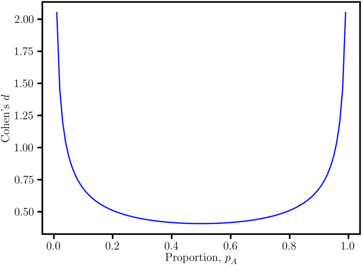
For a fixed value of
rpb, there is a range of (
d,
pA) values (
Fig 1). Alternatively, the variation in (
rpb,
pA) for fixed
d becomes a source of irreproducibility in
rpb because
pA can vary between experiments depending on the data acquisition protocol. This ambiguity explains why researchers have expressed concern about the confounding effect of unbalanced sample sizes on
rpb, and effect size in general [, ]. Furthermore, the binomial
pA
pB dependence originates from the covariance
and variance, Var(
Ic) =
pA
pB. Therefore, the criticism about
pA
pB dependence applies more broadly to the use of the numeric {0, 1} indicator variable. Various researchers have already recommended that the proportions should be equalized,
pA =
pB = 1/2, in to give []
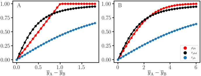
This ‘attenuation-corrected’ coefficient is denoted as
rc in []. The
rpb and
rpbd curves in
Fig 2 provide an illustration of this correction. The one-to-one projective relation between
rpbd and Cohen’s
d is discussed in section 2.4, and the application of
rpbd in rCART is discussed in section 2.5.
Fig 1
Quadratic dependence of the point-biserial correlation coefficient, rpb.
For the fixed value rpb = 0.2, there is a range for Cohen’s d and the sample size proportion, pA. This ambiguity complicates the interpretation of rpb as an effect size measure.
Fig 2
Nonoverlap proportion and point-biserial correlation.
Theoretical curves and estimated values for point-biserial correlation, rpb, nonoverlap proportion, ρpb, and sample size adjusted correlation, rpbd, for simulated data with unequal sample sizes (NA : NB = 15000 : 500) and the difference between mean values, y¯A−y¯B. Compared to rpbd, rpb is attenuated due to the confounding effect of the binomial sampling factor. A: Uniform unit width (σ=1/12) distributions. B: Standard normal (σ = 1) distributions.
2.2 Statistical parameters for point-biserial variation
In this section, we consider the question of how to generate a set of parameters for statistical variation in point-biserial data. The fact that rpb is subject to confounding effects suggests that replacing categorical labels with {0, 1} numeric values is an improper procedure, because the labels acquire arithmetic properties in an ad-hoc way. Instead, we propose a new framework where sort is used as an intrinsic property of both numbers and labels. Suppose there is a machine which generates numbers with labels, (ci, yi), in no particular order, placing them in a data table to produce a point-biserial data set. Then, the table can be sorted using either c or y, to obtain orderings denoted as yc and cy, respectively. As we discuss next, these orderings are associated with statistical parameters, vc and vy, respectively. However, there is no rule that specifies which parameterization, vc or vy, might be preferred. Therefore, we make the following proposition,
Proposition 1. Point-biserial variation is parameterized by the Cartesian product of statistical parameters for the
yc
and
cy
orderings,
The
yc ordering corresponds to sorting the
y data into two sets,
yc ↔ {
yA,
yB}. Then, the statistical parameters for the two sets are associated with a two-component Cartesian product structure, yielding the familiar effect size measures, Cohen’s
d and
rpb as discussed in section 2.3. The
cy ordering is associated with a new nonoverlap measure,
ρpb. The two types of
y-sort, ascending or descending, produce orderings where either {(
ci,
yi)|
yi ≤
yi+1} or {(
ci,
yi)|
yi ≥
yi+1}, respectively. Then, the
c-column corresponds to a
y-ordered string,
cy. The induced order from the
y-sorting is reflected in the degree of mixing of As and Bs in
cy. Next, we sort the data with respect to
c obtaining a maximally ordered string,
cy, where the As and Bs are completely separated.
cM corresponds to the condition where
yA and
yB are disjoint in
R1, which has been characterized as “perfect correlation” []. Our
cy-sorting algorithm requires equal sample sizes,
NA =
NB. When the sample sizes are unequal, a preprocessing step is required. Suppose
NB <
NA. Then, the
yB data are replicated to create a new data set,
yBrep, such that
NBrep =
NA. If the difference in sample size is small, 0 <
NB −
NA <
NB, then a subset of
yB uniformly spaced by rank is replicated. The
yBrep and
yA data are combined to obtain the (
cy,
cM) strings. They constitute a set of joint observations for two categorical variables, which are summarized in a diagonally symmetric 2 × 2 contingency table of the form [[
a,
b], [
b,
a]]. The symmetric form results from the equal sample size condition, which requires that the rows and columns each sum to
NA. Then, the nonoverlap proportion is given by the difference in proportions
where
pa=aa+b, and
pb = 1 −
pa. When
yA and
yB are disjoint, |
ρpb| = 1. The sign of
ρpb is arbitrary because the order of the columns (or rows) of the 2 × 2 table depends on the direction of the sort in
y or
cM. In our implementation, the sign is chosen to be consistent with Cohen’s
d. The
ρpb values in
Fig 2 were obtained using this sort algorithm. The overlap between uniform unit width
(σ=1/12) distributions is an important pedagogical case because the expressions for Cohen’s
d,
rpbd, and
ρpb take a simple form. Geometrically, the overlap (
θU) is given by a rectangle with area
θU = 1 −
δ for the difference between mean values, with 0 ≤
δ ≤ 1, and
θU = 0 for
δ > 1. The nonoverlap is given by
ρpbU = 1 −
θU =
δ, with 0 ≤
δ ≤ 1. Similarly,
For the overlap of standard normal (
σ = 1) distributions, we obtain
where Φ is the cumulative normal distribution function []. In
Fig 2, we observe that at a large enough
δ,
rpbd is attenuated compared to
ρpb, as expected []. However, for small
δ, the inequality is reversed, i.e.,
rpbd >
ρpb. Nevertheless, there is close correspondence between
rpbd and
ρpb for both the uniform and normal distributions. This is particularly true for highly correlated data where both
rpbd and
ρpb are near 1, and are therefore equivalent. However, in section 3 we demonstrate that when the data are not well correlated, both
rpbd and
ρpb are needed in order to distinguish different forms of point-biserial variation. We conclude that
rpbd and Cohen’s
d serve as measures of the nonoverlap of distributions but are not necessarily equivalent to
ρpb.
2.3 Coordinates for a two-component system of distributed effects
In this section, we discuss the fact that d and ρpb are only two elements of a minimal set of parameters for representing point-biserial variation. The one-to-one correspondence, d ↔ rpbd, will be discussed in section 2.4. Algebraically, vc corresponds to the Cartesian product of statistical parameters for two sets of R1 data, vc=(y¯A,SA2,NA)×(y¯B,SB2,NB). Introducing the center of mass parameter, μ=(y¯A+y¯B)/2, the mean values vector is expressed as
where (1, 1) and (1, −1) comprise the center of mass basis. We note that the generalization for a weighted average is straightforward. A similar decomposition holds for variances
where
Sμ2=(SA2+SB2)/2 and
Sδ2=SA2-SB2. A further reduction is obtained if the variances are homoscedastic,
SA2=SB2, yielding
Sp2=Sμ2, and
Sδ2=0. Finally, we obtain
as a minimal set of parameters for point-biserial variation. However, we observe that
vpb is not unique because functions of the components, {
fi(
vpb,i)}, including linear fractional transformations can be introduced to obtain alternative representations. Mathematics alone is not sufficient to specify a preferred vector basis, which explains why there are alternative effect size measures [, ]. Furthermore,
rpb and Cohen’s
d correspond to perspective functions [] of
vpb and do not account for all of the degrees-of-freedom. Consequently, the practice of using one of these measures to serve as a one-parameter summary of experimental results will be subject to irreproducibility.
The term ‘substantive significance’ has been used to refer to the magnitude of an effect that would be regarded as practically important in a given application []. Suppose functional or engineering requirements are expressed in terms of a vector, h, of system parameters. Then, the utility of an effect would be specified as a mapping, u:h↦R1. The specification of u(h) would account for differences in cost-benefit trade-offs for variation in the {hi} components. The substantive significance for the effect size would be determined by the mapping, u(h) → u(vpb). Without this information, it is difficult to reach a consensus on the merits of an effect size. This explains the criticism of Cohen’s thresholds for small, medium, and large effects as “somewhat arbitrary” [] and suggestions that the significance of the magnitude of an effect size depends on the research question [, , ].
A fundamental limitation arises from the fact that the (δ, μ) center of mass decomposition does not extend to higher dimensions in a straightforward way. Consider the group means vector for three sets, i.e., (y¯A,y¯B,y¯C). The default center of mass parameter is defined as μ=(y¯A+y¯B+y¯C)/3. However, there is no standard procedure for choosing the two additional deviation parameters needed to specify a complete basis. Consequently, the formulation of an effect size measure for multiple group variation is not a well-posed problem, i.e., there is no unique solution []. This explains why Cohen’s d does not generalize to schemes involving more than two groups [] and provides support for previous recommendations to break down ‘complicated hypotheses’, p. 526 [], and ‘reduce any multiple-level or multiple-variable relationship’ into a set of two-variable effect size relationships []. This provides the raison d'être for the development of exploratory methodologies such as CART in high-dimensional data analytics [, ].
2.4 Homogeneous coordinates for Pearson correlation
In the effect size literature, it is accepted practice to distinguish three different types of effect size measure, ‘relationship’, ‘group difference’, and ‘group overlap’ [, ]. In this section, we discuss the fact that this classification is misleading. We have already discussed the fact that Cohen’s d, rpbd and ρpb all serve as measures of nonoverlap (section 2.2). Now, we point out that rpbd and Cohen’s d are two sides of the same coin because relationship and group difference correspond to different coordinate systems for representing fractional variation. Such correspondences are quite useful in exploring statistical dependence in high-dimensional data. Consider a vector (a,b)∈R2. Division by the y-component produces the ratio vector, {α=(α,1)∈P1|α=a/b,b≠0}. Ratios can be distinguished by their representations as points in the projective line, P1. However, normalization of a ratio vector by the Euclidean length, ‖α‖=α2+1, produces the unit vector α^, which is a point in the positive half-circle S+1. Thus, a fractional quantity can be represented as a point in either P1 or S+1. Algebraically, the P1 and S+1 representations are related by linear fractional transformations. In the terminology of projective geometry, a ratio corresponds to a perspective function, P(u, t) = u/t, for vector u []. The scaling invariance property of α is represented by the equivalence relation
with
t ≠ 0. Geometrically, this relation specifies points on the line passing through the origin, (
a,
b) and (
α, 1). The points, (
a,
b)
t, constitute the homogeneous coordinates [] for the line. The homogeneous coordinates concept shows that there is a natural correspondence between ‘relationship’ and ‘group difference’ effect size. Expressing the Pearson product-moment correlation coefficient as the rescaled covariance []
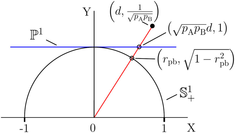
the corresponding projective geometric structure is as summarized in
Table 1. Vector representations for
rpb and
rpbd are also listed, and a geometric visualization for
rpb is shown in
Fig 3. Consequently,
rpbd, Cohen’s
d, and
ρpb each possess
P1 and
S+1 representations and serve as measures of group overlap, as described in section 2.2. Therefore, we conclude that the general classification of effect size as a ‘relationship’, ‘group difference’, or ‘group overlap’ index is misleading. We also observe that the question of the merits of Cohen’s
d versus
rpb in [] is complicated by the fact that these measures correspond to points in different spaces,
P1 and
S+1, respectively. The limitations of
rpb are more easily understood by considering its representation as the vector,
(pApBd,1)∈ℙ1. The binomial factor has a confounding effect, particularly since base rates are determined by the experimental protocol. This is analogous to the confounding effect of the marginal sums on the
ϕ coefficient for a 2 × 2 contingency table (Paper1). Therefore, neither
rpb nor
ϕ meet the criterion for a well-behaved effect size of serving to quantify ‘some phenomenon that addresses a question of interest’ []. In section 2.5, we give an example where
rpb gives nonintuitive results in rCART analysis.
Fig 3
Projective spaces for the representation of point-biserial correlation.
The point-biserial correlation coefficient, rpb, corresponds to the point (rpb,1-rpb2) on the positive half-circle, S+1, and the point (pApBd,1) on the projective line, P1. The homogeneous coordinates (pApBd,1)t for t∈R1 correspond to points on the line through the origin. {pA, pB}: sample size proportions, d: Cohen’s d.
2.5 Point-biserial variation in regression tree analysis
The CART association graph was introduced in Paper1 as a new method for analyzing statistical association in point-biserial data. In this section, we investigate the role of point-biserial variation in rCART, particularly the connection between IGMSE and rpb, and introduce the rCART graph as a new method for analyzing association for (x, y) data. The CART decision tree algorithm creates a decision tree by recursive partitioning of the association between response and independent variables [, ]. Each node of the tree corresponds to a binary partition of the range of an independent variable. In standard implementations, the partition parameters for a node are determined by maximizing the information gain (IG) for the response variable in an exhaustive search of associations over all independent variables. The rCART implementation is of particular interest because it involves the analysis of point-biserial variation. In each iteration, the set of statistics obtained for partitions of an independent variable constitutes a CART association graph []. For the partition value xj∈R1, the data for a node (V) are divided into two subsets, i.e., VA = {(xi, yi)|xi ≤ xj} and VB = {(xi, yi)|xi > xj}, from which data vectors {yA, yB} are obtained. Alternatively, if xj is categorical, the subsets are specified using matching criteria VA = {(xi, yi)|xi = xj} and VB = {(xi, yi)|xi ≠ xj}. The standard rCART impurity measure is the mean square error for the response, MSE(y)=∑i(y¯-yi)2/NV, where NV is the sample size and y¯ is the mean []. Then, IG is defined as the parent node impurity minus the weighted impurities for the subsets
where
pA and
pB are the sample size proportions. Partitioning the sum of squares, MSE(
y), gives [, ]
Substitution for MSE(
y) in gives
Thus, IG
MSE(
yA,
yB) is equivalent to
rpb2 with
Sp = 1 (
Table 1); IG
MSE does not account for the variation in
Sp. To the best of our knowledge, this connection between IG
MSE and
rpb has not been reported previously. We conclude that the analysis of point-biserial variation serves as the basis for rCART, and we use the terms ‘effect size’ and ‘information gain’ interchangeably. The
xj partition produces subsets with sample sizes,
j and
NV −
j for
xj∈R1. An association graph is obtained by searching over all partitions where the sample size proportions,
pj and (1 −
pj), vary over their entire range, producing a large parabolic variation in the
pj(1 −
pj) factor. Thus, an association graph is a convenient way to compare the sample size proportion dependence of effect size measures. In the next section, we demonstrate that
rpb gives misleading results in rCART, while
rpbd and
ρpb produce more intuitive results. However, when the (
x,
y) data are highly correlated and Pearson
r(
x,
y) → 1, the rCART graph becomes a horizontal line or nearly so, because
rpbd ≈
ρpb ≈ 1 for all
xj partitions. Then, the rCART graph and Pearson
r are equivalent representations. Thus, CART methodology is most useful when the data are poorly correlated, which includes population studies where system performance is determined by trade-offs between multiple factors. Typical applications include GWAS, and other high-dimensional search problems such as nursing home performance as discussed in the next section.
3 Data analysis and results
In Paper1, we used the publicly accessible Nursing Home Compare (NHC) data [] in CART analysis to demonstrate the importance of adjusting for the dependence on marginal sums for 2 × 2 contingency tables []. In this section, we use a similar NHC data set for a discussion of point-biserial variation and the rCART algorithm. Our objective is to provide a practical demonstration of the limitations of rpb due to the confounding effect of unbalanced sample sizes and to compare the behaviors of rpbd and ρpb. We also discuss the importance of accounting for three degrees of freedom, (rpbd, μ, ρpb), and the use of Monte Carlo methods to estimate the joint distribution of statistical parameters.
3.1 rCART association graphs for NHC quality measures
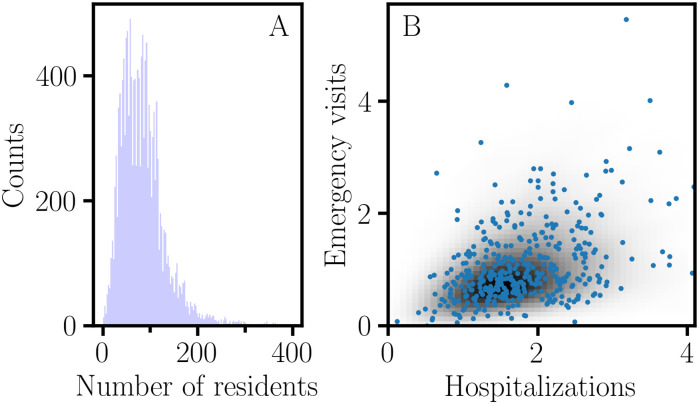
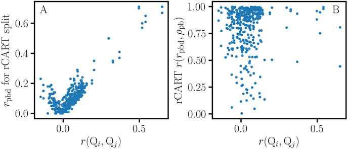
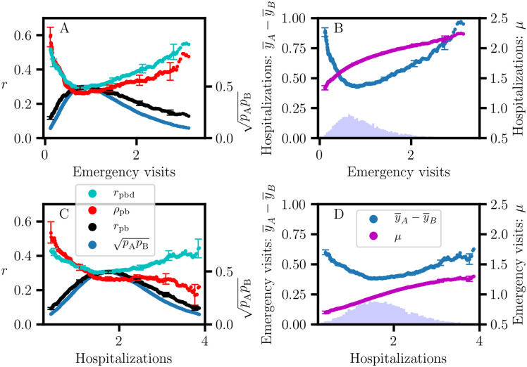
NHC data of the fourth quarter of 2018 were retrieved for 20 quality measures (Qi) for 15341 nursing homes; detailed descriptions of these continuous variables can be found on the NHC website []. A histogram of the nursing home occupancy is shown in Fig 4A. Since performance estimates for nursing homes with low occupancy would be less reliable, a minimum occupancy criterion of at least 50 ‘Average number of residents per day’ was applied to obtain a restricted data set of 11053 nursing homes for further analysis []. Pearson correlation coefficients, r(Qi, Qj), and association graphs were calculated for all pairs of quality measures, {(Qi, Qj)|i ≠ j}. On average, the information gain for the rCART partition is larger when the (Qi, Qj) variables are highly correlated (Fig 5A); the r(Qi, Qj) correlations are distributed with 95% less than 0.16 and a maximum of 0.65. The distribution for ‘Number of outpatient emergency department visits per 1000 long-stay resident days’ (‘Emergency visits’) versus ‘Number of hospitalizations per 1000 long-stay resident days’ (‘Hospitalizations’) with correlation r = 0.37 is skewed, with a long tail towards larger values (Fig 4B). rCART association graphs are shown for the ‘Hospitalizations’ response and ‘Emergency visits’ partition variables (Fig 6A and 6B), and for the reverse, i.e., ‘Emergency visits’ response and ‘Hospitalizations’ partition variables (Fig 6C and 6D). The high correlation between rpb and pApB (r = 0.99) is typical and indicates that variation in the binomial sampling factor overrides the smaller variation in Cohen’s d (). We also note that the graphs for rpb and IGMSE (not shown) are superimposable, as expected from and because the variation in Sp is small. Thus, rpb and IGMSE mainly correspond to the variation in sample size proportion. In general, we observe that the association curves for rpbd and ρpb can be categorized as monotonically increasing or decreasing, or even U-shaped (concave up), depending on how the (Qi, Qj) data are distributed. Here, the U-shaped dependence of rpbd correlates well with δ (r = 0.999) and contrasts sharply with the concave down variation for rpb. Consequently, rpb and rpbd produce very different rCART partitions (Table 2). In Fig 6A, the rpb partition for the split value, xj = 0.8, produces subnodes with comparable sample sizes, NA = 5742 and NB = 4890 (Table 2). It is useful to view this partition from a statistical perspective. As a first approximation, we expect that the majority of nursing homes belong to a broad distribution for average performance. Then, the rpb partition with a split value close to the median, 0.85, is analogous to splitting a normal distribution nearly in half, producing subsets with different mean ‘Emergency visits’ values {0.5, 1.4} that nevertheless correspond to entities with average performance. Thus, rpb and IGMSE produce rCART subsets that are not well distinguished from a functional perspective. In comparison, for rpbd, there are two possible rCART partitions at either low (xj = 0.3) or high (xj = 2.5) split values. Each partition produces a large subset corresponding to a broad distribution for average performance and a much smaller subset for either above- or below-average performance. Thus, rpbd produces more functionally relevant classifications.
Fig 4
Skewed distributions for NHC quality measures.
A. Histogram of ‘Average number of residents per day’ for 15341 nursing homes. B. Two-dimensional Gaussian kernel density estimate of the distribution of ‘Number of outpatient emergency department visits per 1000 long-stay resident days’ (‘Emergency visits’) versus ‘Number of hospitalizations per 1000 long-stay resident days’ (‘Hospitalizations’), with correlation r = 0.37.
Fig 5
The relation between rpbd and ρpb in rCART.
These graphs display data obtained from association graphs for 380 pairs of quality measures, {(Qi, Qj)|i ≠ j}. A. rpbd effect size for rCART split versus correlation r(Qi, Qj). On average, the largest information gain is obtained when the response and partition variables are highly correlated. B. Correlation r(rpbd, ρpb) between effect size and r(Qi, Qj) for association graphs. There is good correlation between rpbd and ρpb in many cases, but there are exceptions.
Fig 6
rCART association graphs for effect size.
A,B: ‘Hospitalizations’ response versus ‘Emergency visits’ partition variables, with correlation r(rpbd, ρpb) = 0.93. C,D: ‘Emergency visits’ response versus ‘Hospitalizations’ partition variables, with correlation r(rpbd, ρpb) = 0.49. Bar plot histograms are shown for ‘Emergency visits’ (B inset) and ‘Hospitalizations’ (D inset). rpb: point-biserial correlation coefficient, {pA, pB}: sample size proportions, rpbd: sample size corrected correlation coefficient, ρpb: nonoverlap proportion, (δ, μ): center of mass parameters (y¯A-y¯B,(y¯A+y¯B)/2).
rCART subnode parameters.
| Response variable | Partition variable | Split value | Subnode A | Subnode B |
|---|
| Hospitalizations | Emergency visits | rpbd: 0.3 | 1.8, 0.7, 9909 | 1.2, 0.7, 723 |
| ” | ” | rpb: 0.8 | 2.0, 0.7, 5742 | 1.5, 0.7, 4890 |
| ” | ” | rpbd: 2.5 | 2.5, 0.8, 320 | 1.7, 0.7, 10312 |
| Emergency visits | Hospitalizations | rpbd: 0.7 | 1.0, 0.6, 10137 | 0.5, 0.4, 495 |
| ” | ” | rpb: 1.7 | 1.2, 0.7, 5318 | 0.8, 0.5, 5314 |
| ” | ” | rpbd: 3.3 | 1.5, 1.0, 330 | 1.0, 0.6, 10302 |
The importance of accounting for variation in both degrees of freedom, (rpbd, μ), is illustrated in Fig 6B and 6D. Here, μ is monotonically increasing, and one of the rpbd partitions might be preferred depending on μ. However, this requires an assessment of the cost-benefit trade-offs for (rpbd, μ) variation, which will depend on the particular application. A close correspondence between rpbd and ρpb is observed in many cases, with r(rpbd, ρpb) ≥ 0.8 in 68% of the association graphs (Fig 5B), but there are many cases where they differ depending on how the (Qi, Qj) data are skewed. Fig 6C shows an example of the difference between the ρpb and rpbd curves with r(rpbd, ρpb) = 0.49. The rpbd partition for the lower split value might be preferred because it is associated with higher ρpb, depending on how the cost-benefit trade-off is assessed for (rpbd, ρpb) variation. Consequently, three coordinates (rpbd, μ, ρpb) are needed to distinguish different forms of point-biserial variation. These observations provide support for previous remarks stating that interpreting the magnitude of an effect size as a measure of substantive significance depends on the particular application [, ]. A more precise approach would take into account the multidimensional nature of point-biserial variation and involve the specification of functional or engineering requirements for a relevant vector basis. Then, an analysis of the effect size for the system response could involve separate thresholds for each coordinate. The ability to account for all relevant degrees of freedom is also important in assessing reproducibility. A one-parameter representation using an effect size such as rpbd or Cohen’s d gives an incomplete picture and leads to ambiguous results because of the loss of information.
3.2 Distributed effects in point-biserial variation
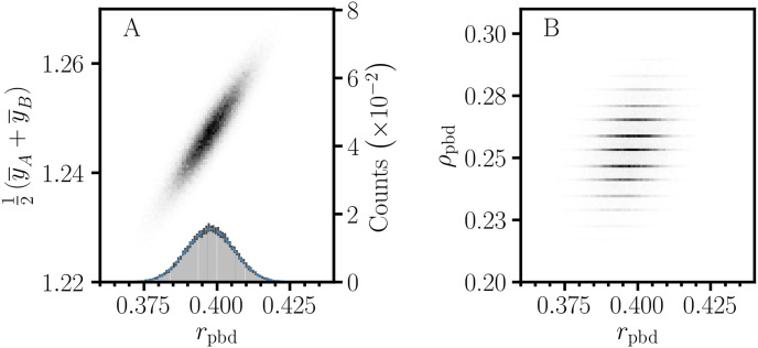
The reproducibility of nursing home performance data depends on stochastic effects in the measurement of patient outcome. Then, the observed data are associated with a distribution of data sets, P(y), and corresponding distributions of the statistical parameters P(vpb) and effect size. The specification of P(y) must be based on a realistic assessment of all sources of error and uncertainty to form an error model for the data, E(y). Then, the determination of the distribution for the effect size requires propagation of the error in P(y). For fractional quantities such as Cohen’s d and rpbd, it is necessary to account for stochastic effects in both the numerator and denominator. However, analytical methods for estimating distributions for ratios [, ], proportions [, ], and correlation coefficients [] are complicated by fractional transformation, a bounded range, and discreteness. Thus, iterative procedures are needed for the analysis of noncentral effect size distributions and estimating confidence intervals for deviations above and below the effect size estimate [, ]. Alternatively, Monte Carlo (MC) methods [, , ] provide a more practical approach to estimating the distribution for the effect size. In an MC simulation, E(y) specifies error parameters for each observed value in the original data. Then, a point-biserial MC data set is obtained by random sampling to produce MC instances for yA and yB. The MC sampling process is repeated many times to obtain a collection of MC data sets to form an estimate, Pi(y). Statistical parameters are calculated for the data sets in Pi(y) to obtain estimates of distributions and histograms for point-biserial effects. Many MC runs are performed to obtain a set, {Pi(y)|1≤i≤NMCruns}, which allows the determination of the degree of convergence for the MC simulation. However, the information needed to construct an error model is not included in the NHC quality measures data. For this demonstration, we provided a rudimentary ‘Emergency visits’ error model, where σi = yi/5. MC simulations for (rpbd, μ) and (rpbd, ρpb) for ‘Emergency visits’ response with ‘Hospitalizations’ rCART split value, 3.3 (Table 2), are shown in Fig 7. The discrete structure of the ρpb distribution is due to stochastic effects in the cy sorting. The separate confidence intervals in Fig 6 for positive and negative deviation from the observed effect size estimate were estimated from the MC distributions. In practical applications, the advantage of the MC method is that it allows detailed simulation of the data acquisition process, including heterogeneity within groups, and specifications for E(y) can include heteroscedasticity, measurement error, and misclassification [, , ].
Fig 7
Monte Carlo simulation of the distribution of stochastic effects for point-biserial variation.
2D histograms of MC distributions for (rpbd, μ) (A) and (rpbd, ρpb) (B) for ‘Emergency visits’ response with ‘Hospitalizations’ rCART split value, 3.3 (Table 2). The 1σ error bars for the rpbd histogram (A inset) serve as an indication of convergence for the simulation; the mean for the normal curve corresponds to the observed rpbd value, 0.398. rpbd: sample size corrected correlation, ρpb: nonoverlap proportion, μ: center of mass parameter (y¯A+y¯A)/2, number of MC runs: 25, samples per MC run: 4000.











 Nonoverlap proportion and the representation of point-biserial variation
