PLoS ONE

Competing Interests: The authors have declared that no competing interests exist.
- Altmetric
Plant phenotyping is a central task in crop science and plant breeding. It involves measuring plant traits to describe the anatomy and physiology of plants and is used for deriving traits and evaluating plant performance. Traditional methods for phenotyping are often time-consuming operations involving substantial manual labor. The availability of 3D sensor data of plants obtained from laser scanners or modern depth cameras offers the potential to automate several of these phenotyping tasks. This automation can scale up the phenotyping measurements and evaluations that have to be performed to a larger number of plant samples and at a finer spatial and temporal resolution. In this paper, we investigate the problem of registering 3D point clouds of the plants over time and space. This means that we determine correspondences between point clouds of plants taken at different points in time and register them using a new, non-rigid registration approach. This approach has the potential to form the backbone for phenotyping applications aimed at tracking the traits of plants over time. The registration task involves finding data associations between measurements taken at different times while the plants grow and change their appearance, allowing 3D models taken at different points in time to be compared with each other. Registering plants over time is challenging due to its anisotropic growth, changing topology, and non-rigid motion in between the time of the measurements. Thus, we propose a novel approach that first extracts a compact representation of the plant in the form of a skeleton that encodes both topology and semantic information, and then use this skeletal structure to determine correspondences over time and drive the registration process. Through this approach, we can tackle the data association problem for the time-series point cloud data of plants effectively. We tested our approach on different datasets acquired over time and successfully registered the 3D plant point clouds recorded with a laser scanner. We demonstrate that our method allows for developing systems for automated temporal plant-trait analysis by tracking plant traits at an organ level.
Introduction
For optimizing any process, it is important to know or observe the current status of the system to optimize. Thus, approaches for observing or monitoring dynamic systems over extended periods of time are of key interest in several disciplines, especially when dealing with complex systems where input-output relations are complex to formalize. In plant sciences and modern agriculture high-resolution monitoring of plants plays an important role [1, 2]. It forms the basis for analyzing crop performance and provides an indicator of the plant stresses. Measuring how individual plants develop and grow over time is often a manual and laborious task. It often even requires invasive methods that harm the crop. For example, the standard approach to measuring the leaf area is to cut off the leaves and scan them with a flatbed scanner. New measurement technologies for measuring and tracking phenotypic traits employing robots and robotic sensors open up new possibilities to automate the process of measuring plant performance [3, 4]. Recent studies [5, 6] showcase the potential of using 3D laser data for computing geometric plant traits with high fidelity. Agricultural robots equipped with such laser scanners can acquire 3D plant data at a large scale and facilitate high-resolution phenotyping. This is a step forward for scaling up phenotyping from plants grown in a greenhouse to the level of plots and maybe even fields.
Laser scanners and RGB-D cameras, i.e., sensors that can measure the 3D geometry of objects, are commonly used sensors to perceive both static and dynamic environments. Especially in robotics, this is a key task that most mobile systems rely on [7–9]. Extending such robotic-inspired approaches to the agricultural setting, however, is not always straightforward. One of the challenges in this context is to develop techniques that can robustly deal with growing objects, changing appearance, the development of new organs causing changes in the topology as well as non-rigid deformations caused by external factors such as sunlight, wind, gravity, etc. This is illustrated in Fig 1 where we perceive these large changes in the time-series data of two plant types which were recorded with a laser scanner recorded over a period of two weeks. Typically, point cloud registration is performed using iterative closest point-based approaches [8]. These approaches, however, are often unable to capture the deformations in the object and are prone to divergence due to new or missing plant organs. In this paper, we investigate the means to account for the growth and the non-rigid deformations that the plants undergo.

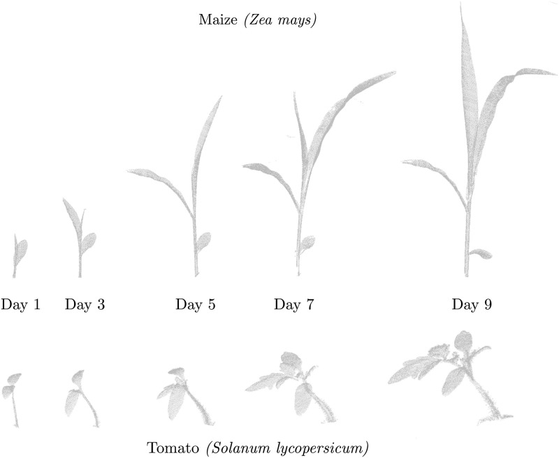
A time-series of 3D point clouds of two plants (maize (top) and tomato (bottom)) captured during its growth.
Our goal is to develop techniques for automatically registering such 3D scans captured under challenging conditions of changing topology and anisotropic growth of the plant.
The main contribution of this paper is a fully automatic registration technique for plant point clouds which have been acquired over time. We propose to use the skeleton structure of the plant to drive the registration process as it provides a compact representation of the plant by capturing its overall shape and topology. In this paper, we propose a method for extracting the skeletal structure along with semantic information to perform the data association step. We classify each point of the plant as a leaf or stem point, a further clustering allows us to compute individual leaf instances. We then determine correspondences between plant skeletons using a hidden Markov model. These correspondences in turn allow us to estimate parameters, which are able to capture the deformation and the growth of the plant skeleton. We then transfer the deformations estimated on the plant skeletons to the whole point cloud to register the temporally separated point clouds. Using these registration parameters, we are also able to interpolate over the registration parameters to obtain an estimated point cloud at a time instant in-between the actual acquisition times.
In sum, our approach is able to (i) register temporally separated plant point clouds by explicitly accounting for the growth, deformations, and changes in the plant topology, (ii) exploit the skeletal structure as well as semantic information computed from the data, (iii) find correspondences between the different organs of the plant and track plant growth parameters over time, (iv) demonstrate reliable registration results on long-term datasets of two types of plants captured using a 3D laser scanner mounted on a robotic arm.
Related work
Phenotyping plays an important role in plant sciences. Traditionally, a lot of the activities required substantial manual work. Over the last decade, however, automated plant phenotyping has been receiving increasing interest, also in other disciplines such as robotics [10, 11] or computer vision [12–14]. One relevant aspect in this context relates to obtaining relevant features of plants, often referred to as phenotypic traits, in an automated manner [2, 15]. Several phenotyping systems [1, 16, 17] have been developed for greenhouse environments and are also available commercially [18, 19]. Other systems such as [20–24] have been designed to acquire plant data directly from the fields or estimate information about plants for management actions [25–28].
These phenotyping systems have been used for several applications such as plant growth monitoring [5], drought stress analysis [29], canopy cover estimation [30], horticulture [31, 32] etc. Several approaches [33–37] aim at obtaining traits at a coarse resolution over the entire field using image data captured from UAVs as well as from ground robots. More recently, 3D laser data has been used in many agricultural applications such as [38–40] and analyzed to obtain phenotypic traits with high fidelity [5, 6, 41]. Li et al. [42] and Paproki et al. [43] analyze time-series point cloud data to detect topological events such as branching, decay and track the growth of different organs. While both works emphasize obtaining phenotypic traits at an organ level, our focus in this paper is on developing basic techniques for matching as well registering temporally separated scans of individual plants using the whole point cloud data. This technique forms the basis for tracking phenotypic traits over time.
Several approaches in the past have attempted to leverage the topological structure of the object to drive the registration process, primarily in the field of human motion tracking [44–46]. A large number of techniques exist for extracting skeletons from 3D models, also known as skeletonization. The skeleton structure of the model is then used for different applications such as animation, tracking, surface reconstruction, etc. Huang et al. [47] use local L1-medial points to compute the skeleton curve for an unorganized point cloud, while Tagliasacchi et al. [48] propose the idea of a generalized rotational symmetry axis of the model which exploits the normal information as well. Recently, Wu et al. [49] proposed a technique using Laplacian point cloud contraction to extract skeletons of maize point clouds. A detailed state-of-the-art review for extracting skeletons of 3D objects is given in [50]. In contrast to these approaches, we exploit both supervised and unsupervised machine learning techniques to compute the skeleton curve for the plant point clouds. In this process, we classify the plant into stem and leaf points, cluster them together as individual organs and use this semantic information for computing the skeleton structure effectively.
Exploiting semantic information of the plant for extracting the skeleton structure is quite helpful. While a large corpus of literature exists for classification in 2D images, the number of approaches that operate on 3D point clouds is rather small. Paulus et al. [51] propose an SVM-based classifier that relies on a surface histogram to classify each point in a 3D point cloud as leaf or stem. The recent approach by Zermas et al. [52]use an iterative algorithm called randomly intercepted node to tackle the same problem. Sodhi et al. [53] use 2D images to extract 3D phytomers, namely fragments of the stem attached to a leaf for leaves detection. Shi et al. [54] propose a multi-view deep learning approach inspired by Su et al. [55] to address the organ segmentation problem, while Zermas et al. [56] uses a skeletonization approach to segment leaf instances. Our approach builds upon the work of Paulus et al. [51] and additionally groups the leave points with an unsupervised clustering algorithm to extract leaf instances. In this way, we achieve an organ segmentation exploiting labeled data for the leaves. We use this in turn as the basis for our registration approach across plant point clouds.
Recent developments for segmenting point cloud data using deep-learning techniques are promising. Several methods have been proposed to segment point clouds, among which PointNet [57]and PointNet++ [58] are often considered as milestones. Several architectures using special convolution operations designed for point clouds such as KPConv [59]provide state-of-the art segmentation results. However, a common requirement for many such techniques is the availability of large-scale labeled datasets. In our application where we are using high resolution plant point cloud data, training datasets at such scale are not available as of yet. Moreover, in this work we essentially use the segmentation results to generate a skeleton from the point-cloud. Since, all other steps in the registration process are designed to cope with imperfections in the skeleton structure, having a precise segmentation for the point cloud is not critical for this approach. As a result, we did not investigate the use of 3D deep learning networks in this work. These techniques can form the basis for segmentation task as opposed to the use SVM as done in this work.
Registering point clouds is a common problem in a lot of disciplines and multiple techniques have been proposed for laser-based or RGB-D-based mapping systems [8, 9, 60]. These techniques work under the assumption the objects being registered only undergo rigid motion. The techniques have been extended by relaxing the rigidity assumption and several non-rigid registration techniques such as [61–63] aim at capturing the deformation in the object. Approaches such as [64–68] aim at reconstructing scenes in an online fashion either in the presence of dynamic objects or deformations. Such approaches typically operate on scans captured at a high frame rate (10-30 Hz) and thereby deal with rather small deformations in between consecutive scans. This assumption is violated for the point cloud data considered here. In our application, the plants are usually scanned at a comparably low frequency (once per day) and thereby showing larger growth and deformations in between consecutive scans. In addition, the problem becomes even more difficult if the object changes its appearance and topology over time. Zheng et al. [69] propose an approach to register 3D temporal point clouds of objects by exploiting skeleton structures. In this paper, we build upon their formulation and integrate it within an improved data association approach which accounts for the topology and the semantic of the plant. We then use these data associations to register temporally separated 3D plant point clouds within an iterative non-rigid registration scheme.
This paper extends our previous conference paper [70] in several ways. First, the prior work required a manually provided skeletonization of the plants, while in this paper, we estimate it from sensor data. Second, we estimate semantic information about the plant organs and exploit this estimate to compute a high-quality skeleton and improve the data association between point clouds. Furthermore, we substantially extended the discussion of related work and provided additional experiments for maize in addition to tomato plants. All these claims are backed up through the experimental results presented in this paper. The implementation of our approach is available at: https://github.com/PRBonn/4d_plant_registration.
Material and methods
Proposed approach to plant point cloud registration
Our approach operates on a time-series of 3D point clouds of plants. Our registration procedure starts with extracting a skeleton along with the organ level semantics for each point cloud. The skeletons are undirected acyclic graphs, which represent the topology or the inner structure of the plant. Each node contains the x, y, z coordinates of its position, a 4x4 affine transformation matrix T to describe the local transformation, and a semantic class label as attributes. The skeletons are extracted from the point cloud data and are often imperfect. This fact is taken into consideration during the registration procedure. We also operate directly on the ordered point clouds and do not require a mesh structure or other cues such as the normals providing the inside-outside information of the surface. The skeleton structures allow us to compute data associations between temporally separated 3D scans and use these correspondences to perform an iterative procedure which registers the plant scans obtained at different times. Finally, the registered skeletons can be used to deform the complete point cloud, e.g., the point cloud from time step t1 deformed to time step t2. The overall registration scheme is summarized in Alg. 1 and will be explained in detail in the following sections.
Algorithm 1 Skeleton-driven iterative non-rigid registration procedure
1: ⊳ Input point clouds
2:
3:
4:
5:
6:
7: while
8:
9:
10:
11:
Extracting the skeletal structure along with semantics
The first step of our approach is to extract the skeleton structure
After the model is trained, we use it to predict the semantics (category) for all the remaining point clouds of the sequence. Once the classification step is complete, we perform a clustering step in order to find the individual leaves or the stem as unique instances. We perform the clustering using the density-based spatial clustering algorithm [73]. It uses the x, y, z coordinates of the points to obtain an initial segmentation, which is then refined by discarding small clusters and assigning each discarded point to one of the remaining clusters based on a k-nearest neighbor approach.
At this stage, each point in the point cloud is assigned to an organ, namely to the stem or to one leaf instance. We then learn keypoints for each organ using self-organizing maps [74]. These keypoints would form the nodes of the skeleton structure. Self organizing maps are unsupervised neural networks using the concept of competitive learning instead of back-propagation. They take as input a grid that organizes itself to capture the topology of the input data. Given an input grid


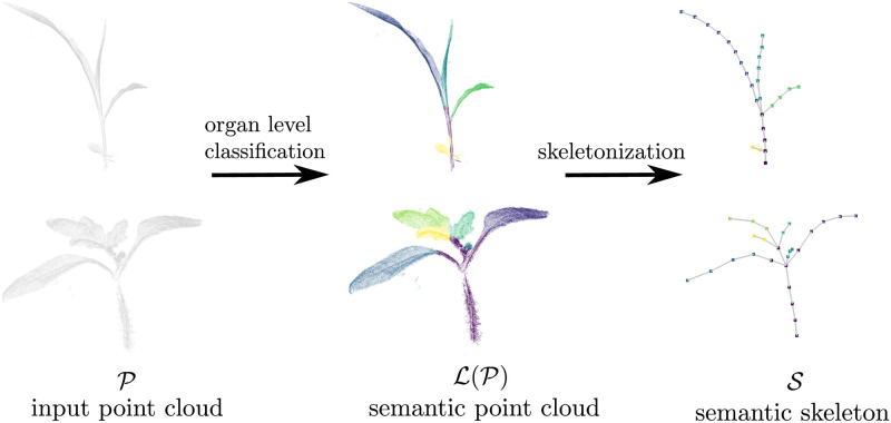
Extracting skeletal structure for using semantics of the plant.
The figure illustrates the skeletonization pipeline for a maize (top) and tomato (bottom) plant scan. Note that for the tomato plant, we classify individual leaflets (green + yellow + light-blue) as separate instances rather than as an individual leaf. The leaflets can be combined into a single leaf in case this distinction is not desired/required for the application.
Estimating skeletal correspondences
Before data from any 3D objects can be aligned, we need to establish the data associations between the sensor readings, i.e, estimating which part of cloud
In this data association step, we estimate correspondences between two skeletons by exploiting their geometric structure and semantics, which are computed using the approach described in the previous section. As the skeleton structure and the semantics are estimated from sensor measurements, it might suffer from several imperfections. To cope with these imperfections in the individual skeletons and inconsistencies between them, we use a probabilistic approach to associate the skeleton parts as opposed to graph matching approaches, which typically do not tolerate such errors well. We, therefore, formulate the problem of finding correspondences between the skeleton pair (
The unknowns or the hidden states of the HMM model represent all the potential correspondences between the nodes of the two skeletons. In addition, we also add a so-called “not matched state” for each node to the HMM to account for the situations in which the node may have no correspondences at all. This happens, for example, when nodes belong to new organs that were not present before or when new nodes emerge on the curve skeleton due to the plant growth. As required in a HMM formulation, we need to define the emission cost Z and the transition cost Γ. The emission cost Z describes the cost for a given hidden state (correspondence) to produce a certain observation. In our case, the observations are the sequence of nodes of the first skeleton

The transition cost Γ describes the cost involved in transitioning from one hidden state cij to another ckh. This can be treated as the cost involved in having ckh as a valid match given that cij is a valid match as well. We define this cost as:

Once the emission and transition costs are defined, we compute the correspondences between the skeletons by performing inference on the HMM. The result is the most likely sequence of hidden variables, i.e., the set of correspondences between

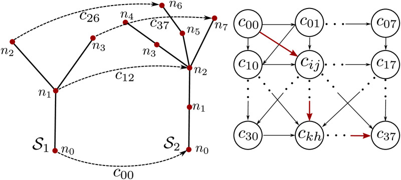
Left: Skeletal matching for an example pair of plant point clouds with the variables involved. Right: Hidden Markov model (HMM) used for correspondence estimation. We only show a subset of the hidden variables, i.e. the potential correspondences, in the HMM. The red line depicts the sequence of best correspondence estimated by the Viterbi algorithm. This produces the correspondences between
Computing skeletal deformation parameters
In this step, we compute the registration parameters between
To model the deformations between the plant scans, we attach an affine transformation Ti to each node ni of the skeleton

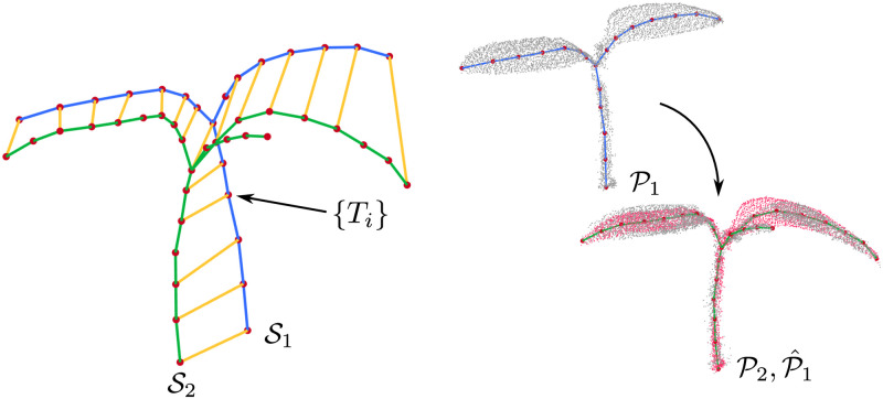
Left: Registering the skeleton pair involves estimating the deformation parameters attached to the nodes of the source skeleton
We define the objective function of the optimization problem as a combination of the three energy terms. The first term Ecorresp is defined as:

The second energy term Erot captures how close the estimated affine transformation is to a pure rotation and it determines the smoothness of the deformation. We define Erot as:

We also define a regularization term Ereg as:


We use the weights wcorresp = 100, wrot = 10, and wreg = 1 for all the example in our datasets. The weights have been chosen such that the cost due to each component of the loss is in the same order of magnitude. We employ the Gauss-Newton algorithm to solve the unconstrained non-linear least squares problem [77]. We use the Cauchy robust kernel [78] for the error residuals belonging to Ecorresp as this prevents incorrect correspondences to influence the optimization process. The robust kernel automatically downweights potentially wrong correspondences, which have large residuals. The approach is related to the formulation by Sumner et al. [63] for estimating deformation parameters for surfaces parametrized as triangular meshes. In our case, we adapt the energy terms to reflect the constraints valid for deformation between curve skeletons as opposed to surfaces. Furthermore, the approach by Sumner et al. [63] is not able to fully constrain the nodes which have a degree smaller than 3, but is essential for registration of curve skeletons.
Point cloud deformation
Traditional approaches to point cloud registration assume rigid objects. In this case, the alignment results in the execution of a 6 degree of freedom transformation consisting of rotations and translations. This, however, is substantially different in our case. To obtain the final registered point cloud
For each point


Iterative non-rigid registration procedure
We use the steps from the previous sections to formulate an iterative approach to register the point cloud pair
Interpolating point clouds of plants
In addition to registering the plant scans recorded at different times, we would also like to interpolate how the plant may be deformed at an intermediate time in between the actual acquisition times. This may allow for increasing the time between the recordings and doing further analysis on the interpolated point clouds. We compute the deformed point cloud by interpolating the deformation parameters T estimated between the two registered scans. To obtain a smooth interpolation, we first decompose of the estimated affine transformation T into scale/shear transformation Ts, pure rotation TR, and a pure translation Tt using the polar decomposition approach described by Shoemake [79] and is given by:

We then linearly interpolate Ts and Tt to obtain the transformation at time t. For interpolating TR, we use the spherical linear interpolation described by Shoemake [80].
Computing phenotypic traits
In this work, we compute different phenotypic traits for both the stem and leaf instances. In particular, for the stem class, we compute stem diameter and stem length, whereas for the leaf class, we compute the leaf length and area. We choose these traits as examples, and other geometric traits that use the area or shape of the organs can be computed and tracked over time as well.
The stem and leaf length can be easily computed from the geometric information of the semantic skeleton: The stem/leaf length is just the sum of the lengths of the edges of all nodes of a particular instance.
For computing the stem diameter sd, we first assign each point in the point cloud classified as stem to the closest node on the skeleton. Then, we compute the main axis of the data distribution in the neighboring region of the selected node using a standard singular value decomposition (SVD) approach. We can then compute the stem diameter with respect to the main axis of the considered neighborhood. The stem diameter sd is obtained as:

We compute the leaf area la by exploiting the SVD to estimate the main plane A of the points associated with each node. This gives us the leaf area la as:

Experimental results
Dataset description
We evaluate our approach on time-series 3D point cloud data of three sample plants of maize (Zea mays) and tomato plants (Solanum lycopersicum). The scans were recorded using a robotic arm (Romer Absolute Arm) [81] equipped with a high precision laser scanner. The dataset was recorded daily over a period of 10 days. The plants have been scanned in manner so as to minimize self occlusions whenever possible. The point cloud data undergoes a pre-processing step where all the points which do not belong to the plant are removed, for example the points belonging to the soil and the pot. The datasets cover substantial growth of the plants, starting from the 2 cotyledons (i.e. seed leaves) at the start to around 8 leaflets (2 cotyledons + 2 leaves) for the tomato plants, and 1 to 4 leaves for the maize plants. The plants undergo substantial leaf and stem growth, and includes several branching events till the end of the dataset acquisition period as illustrated in Fig 1. The height of the tomato plants reaches up to 150 mm and the maize plant reaches over 400 mm. The data used in the paper is available at: https://www.ipb.uni-bonn.de/data/4d-plant-registration/.
Semantic classification of plant point clouds
In the first experiment, we evaluate the performance of our approach for organ level semantic classification. The classification system has been trained on two randomly selected point clouds from each datasets. All the remaining point clouds in the sequence are used as test datasets. The ground truth information for both the training and test sets have been generated manually by human users. We show the qualitative results computed by our approach by visualizing the semantic instances for some point clouds from the two datasets in Fig 5. Each stem and leaf instance is visualized with a different color. We can visually inspect the stem and the leave instances throughout the temporal sequence, and see that the classification is successful for instances despite their size and shape changing over time. The colors of same leaf instances do not persist over the temporal sequence since the data associations between them have not been computed at this stage.

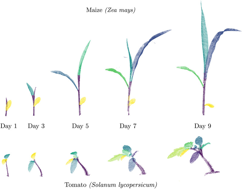
Semantic classification of maize (top) and tomato (bottom) point clouds.
Each stem and leaf (or leaflet) instance is visualized with a different color. Note that the colors of same leaf instances do not correspond over time, as data associations have not been computed at this stage.
We also perform a quantitative evaluation of the classification performance of our classification approach by computing standard metrics [82] such as precision

| Dataset | Stem | Leaf | Instances | |||||||||
|---|---|---|---|---|---|---|---|---|---|---|---|---|
| mean | min | max | std | mean | min | max | std | mean | min | max | std | |
| Maize | 86.3 | 74.5 | 99.6 | 8.6 | 95.5 | 93.6 | 99.4 | 2.2 | 94.4 | 91.9 | 99.6 | 2.7 |
| Tomato | 89.6 | 68.6 | 99.2 | 9.6 | 97.9 | 96.9 | 99.0 | 0.9 | 83.4 | 59.8 | 99.7 | 15.4 |

| Dataset | Stem | Leaf | Instances | |||||||||
|---|---|---|---|---|---|---|---|---|---|---|---|---|
| mean | min | max | std | mean | min | max | std | mean | min | max | std | |
| Maize | 85.7 | 48.6 | 99.1 | 16.3 | 92.9 | 89.1 | 99.8 | 3.3 | 94.7 | 91.3 | 99.6 | 3.1 |
| Tomato | 92.2 | 60.6 | 99.4 | 11.4 | 96.5 | 74.0 | 99.6 | 8.3 | 78.2 | 66.6 | 99.4 | 11.2 |

| Dataset | Stem | Leaf | Instances | |||||||||
|---|---|---|---|---|---|---|---|---|---|---|---|---|
| mean | min | max | std | mean | min | max | std | mean | min | max | std | |
| Maize | 80.0 | 47.8 | 94.6 | 12.7 | 94,6 | 88.9 | 97.4 | 2.5 | 94.0 | 91.0 | 97.6 | 2.3 |
| Tomato | 82.6 | 60.6 | 92.2 | 10.4 | 93.4 | 73.9 | 99.0 | 7.8 | 69.1 | 51.4 | 98.7 | 15.7 |
Despite these accurate results, it is worth noticing that the ability of the SVM to classify stem points is lower on the maize dataset than on the tomato dataset. This is due to a smoother transition between stem and leaves in the maize plants. In contrast, the performance of the clustering is higher on the maize dataset. This behavior can be explained by looking at how leaves develop in the two species. While for the maize plants there is a clear separation between individual leaves, this separation is not as clear for the leaves in the tomato plants. For reference, we have shown the ground truth labels for two example plants used in the evaluation of semantic classification in Fig 6.

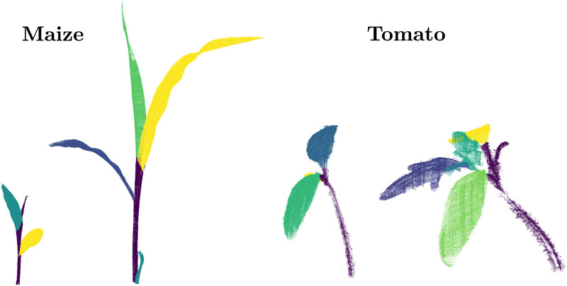
Example ground truth labels used in the evaluation of semantic classification of maize (left) and tomato (right) point clouds.
The instance wise labels for each plant organ have been manually annotated by a human user.
4D registration of plant point clouds
In the second experiment, we demonstrate that our approach successfully registers time-series point cloud data for two plant types. We use the same weights for our registration procedure as described in the methods section for all scan pairs (both tomato and maize datasets) at different growth stages. We also perform a quantitative evaluation of the accuracy of the registration pipeline. Fig 7 illustrates the results of the registration procedure for two example scan pairs from the maize (top) and the tomato (bottom) datasets. For both examples, we show the input point clouds (

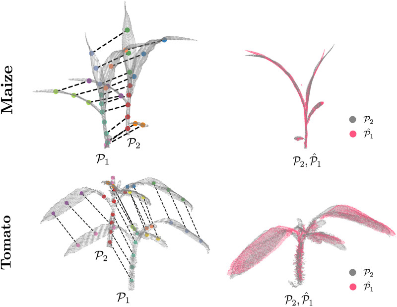
4D registration of a point cloud pair scanned on consecutive days for maize (top) and tomato (bottom) plant.
The left column shows the two input point clouds (
Further, we quantitatively evaluate the accuracy of our registration pipeline by registering all consecutive scans of the two datasets. First, we compute the accuracy of our skeleton matching procedure by computing the percentage of correspondences estimated correctly. We define the correct correspondences as those which belong to the same organ (i.e., the same leaf or the stem) in the skeleton pair as there is no unique way to define a correct correspondence due to the growth in the plant. We manually label the different organs of the plant with a unique identifier to provide the ground truth to compute this metric. For our tomato datasets, we obtain an average of 95% correct correspondences between consecutive skeleton pairs with most pairs having all the correspondences estimated correctly. For the maize dataset, we obtain 100%of the correspondences between consecutive days correctly. Similarly, we also evaluated the accuracy of the correspondence estimation between skeleton pairs with 2 and 3 days apart from each other. For the tomato dataset, we obtain again an average of 95% correspondences with scans taken 2 days apart, whereas this falls down to 88% with scans taken 3 days apart. Again for the maize dataset, we obtain all the correspondences correctly both with skeletons taken 2 and 3 days apart. The higher accuracy for the maize plants is likely due to the simpler shape of the plant as compared to the tomato plants.
Secondly, we evaluate the accuracy of the estimated registration parameters by computing the error between the deformed source point cloud

As this registration measure may be susceptible to some degenerate cases, an extreme case being all points
As a baseline comparison, we assume a rigid transformation for the whole point cloud between consecutive scans and computed the transformation with a standard ICP approach. The average error ereg for this experiment is 35 mm and the maximum error is 166 mm. The large errors using a rigid transformation assumption are both due to the plant growth and in some cases, the ICP procedure diverging completely. This indicates that a rigid transformation assumption is inadequate and a non-rigid registration procedure is required to capture the growth and movement of the plant.
We visualize the registration error as a heat map for the two example point cloud pairs in Fig 8. The heat map is projected on

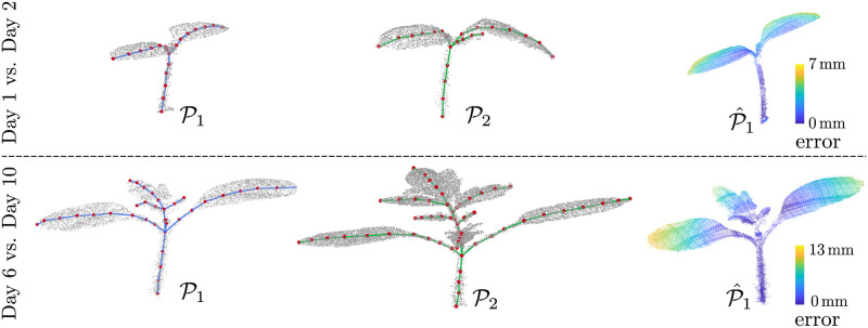
Visualizing registration error.
We visualize the registration error as a heatmap for two pairs of tomato plant scans, Day 1 vs. Day 2 and Day 6 vs. Day 10. Blue represents low registration error whereas yellow represents a larger error.
Temporal tracking of phenotypic traits
In this experiment, we show that the spatial-temporal registration results computed by our approach allows us to compute several phenotypic traits and track them temporally. We compute the area la and length ll for leave instances and the diameter sd and length sl of the stem for each point cloud in the temporal sequence as describe previously, and associate it over time using the data associations estimated by our approach during the registration process. The tracking results for the three sample plants from the maize and tomato datasets are visualized in Fig 9. The first two columns in Fig 9, track the leaf area and leaf length over time. Different shades of blue and green in these plots represent individual leaf instances. In addition, we can also detect certain events, which mark a topological change in the structure of the plant such as the appearance of a new leaf. These events can be recognized from the leaf area or leaf length plots in Fig 9 whenever a new line rises up from the zero level. For example, for the first plant in the maize dataset, a new leaf emerges on day 2, 3, and 6. In the rightmost column in Fig 9, we see that stem length and diameter for both the datasets increase considerably over the data acquisition period. Such phenotypic information can also be used to compute the BBCH scale [83] of the plant, which is a growth stage scale and provides valuable information to the agronomists.

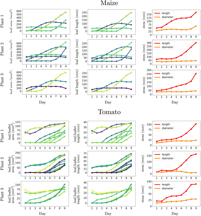
Tracking phenotypic traits for individual organs of the plant.
Our registration procedures allows us to track the growth of the stem and different leave lengths over time and detect topological events such as the emergence of new leaves. Different shades of blue and green in these plots represent individual leaf instances in the first two columns. The orange and red represent the length and diameter of the stem respectively.
Temporal interpolation of plant point clouds
In the last experiment, we demonstrate that the registration results can be used to interpolate the point clouds at intermediate points in time, i.e., in between the actual acquisition times of the scans. The ability to interpolate is useful for analyzing properties of the plants even when actual measurements are not available. It allows us to predict both, the motion and growth at intermediate time intervals. We visualize the interpolated point cloud at three time instances


Interpolation of point clouds at intermediate time intervals.
Point clouds (gray) at time t − 1 and t come from actual scan measurements whereas the points clouds (pink) at time instants
Summary and conclusion
In this paper, we presented a novel approach for spatio-temporal registration of 3D point clouds of individual plants. The proposed method works for raw sensor data stemming from a range sensor such as a 3D LiDAR or a depth camera. The processing of the sensor data happens in a fully automated fashion without manual intervention. We implemented and evaluated our approach on datasets of tomato and maize plants presenting challenging situations and supported all claims made in this paper. The experiments suggest that our registration approach can be used as a basis for tracking plant traits temporally and contribute towards automated phenotyping. Furthermore, we released the code of our approach as open-source software.
Our approach works as follows: First, it estimates the skeletal structure of the plant, exploiting also a point-wise classification approach to compute a skeleton representing the plant. This skeleton structure including the semantic information is used to find reliable correspondences between parts of the plant recorded at different points in time using a novel data association approach that relies on a hidden Markov model. It allows for estimating a global association between the skeletons of the plants extracted from point clouds recorded at different points in time. As our results showcase, this approach can deal with changing appearance and changing topology of the 3D structure of the plant. This is an essential capability to form a robust alignment of the 4D data, i.e., of 3D geometry and time. Given the data associations, we explicitly model the deformation and growth of the plant over time using multiple affine transformations associated with the individual nodes of the skeleton structure. In this way, individual parts of the plant are transformed using different affine transformation modeling the different growth along the plant. The parameters for these transformations are estimated using a robust least-squares approach including regularizations. Given the resulting parameters, we can align 3D scans taken at different points in time and transform them according to the growth. This, in turn, allows us to estimate basic phenotypical parameters such as leaf area, leaf length, as well as stem diameter or length and track their development over time in an automated fashion.
Acknowledgements
We thank Heiner Kuhlmann and his group at the University of Bonn as well as Stefan Paulus for providing the 3D scans of the plants used in this paper.
References
1
2
3
4
5
6
7
8
9
10
11
12
13
14
15
16
17
18
19
20
21
22
23
24
25
26
27
28
29
30
31
32
33
34
35
36
37
38
39
40
41
42
43
44
45
46
47
48
49
50
51
52
53
54
55
56
57
58
59
60
61
62
63
64
65
66
67
68
69
70
71
72
73
74
75
76
77
78
79
80
81
82
83
 Registration of spatio-temporal point clouds of plants for phenotyping
