PLoS ONE

Competing Interests: NO authors have competing interests.
- Altmetric
Risk in finance may come from (negative) asset returns whilst payment loss is a typical risk in insurance. It is often that we encounter several risks, in practice, instead of single risk. In this paper, we construct a dependence modeling for financial risks and form a portfolio risk of cryptocurrencies. The marginal risk model is assumed to follow a heteroscedastic process of GARCH(1,1) model. The dependence structure is presented through vine copula. We carry out numerical analysis of cryptocurrencies returns and compute Value-at-Risk (VaR) forecast along with its accuracy assessed through different backtesting methods. It is found that the VaR forecast of returns, by considering vine copula-based dependence among different returns, has higher forecast accuracy than that of returns under prefect dependence assumption as benchmark. In addition, through vine copula, the aggregate VaR forecast has not only lower value but also higher accuracy than the simple sum of individual VaR forecasts. This shows that vine copula-based forecasting procedure not only performs better but also provides a well-diversified portfolio.
Introduction
In finance and insurance, one of the major and challenging issues is managing quantitative risk, specifically forecasting future risk. Risk forecast is not only important for reserving capital but also for anticipating the worse risk. Risk in finance may come from (negative) asset returns whilst, in insurance, a typical risk is a payment loss. It is often that we encounter several (dependent) risks, in practice, instead of a single risk. Dependent random risks or losses occur in many applications and have challenging statistical features, see e.g. Embrechts et al. [1, 2], Gräler et al. [3], McNeil et al. [4], Naifar [5], Patton [6], Trabelsi [7], Usman et al. [8] and Zhang et al. [9].
There are several interesting topics that relate to dependent risks. The first one is construction of dependent risks either as an aggregate risk model or a multivariate risk model, see e.g. Kim and Kim [10]. The second topic lies on the fact that dependent risks have a technical problem with regard to finding an exact form of distribution function (cdf) or probability function (pdf). Both topics above eventually bring us to learn and employ a more sophisticated method in dependent risks namely copula. Copula is a system that does not only accommodate either non normal or unidentical marginal distributions into a uniform distribution but also simplify number of parameters of a joint distribution. Meanwhile, a more step method than a copula is vine copula. It is also a system that constructs pair-copula with high flexibility when decomposing conditional distribution, e.g. Aas et al. [11] and Trucíos et al. [12]. Furthermore, vine copula provides us informative and complete dependence structure. It is well known that understanding dependence is an important step to make strategy on diversification.
Modeling dependence through vine copula approach is basically aimed to broaden flexibility of dependence structure among random risks, compared to classical dependence measures of Pearson’s ρ and Kendall’s τ or even copula. The recent use of vine copula modeling may be found in (energy) economic and finance applications. For instance, Mejdoub and Ghorbel [13] investigated conditional dependence between oil price and renewable energy stock prices and considered threshold Generalized Autoregressive Conditional Heteroscedastic (GARCH) model, see also Trabelsi [7] for tail risk dependence between oil and stocks of oil-exporting countries. Kumar et al. [14] examined conditional dependence among not only energy commodities but also agricultural and precious metals commodities. Furthermore, Çekin et al. [15] studied dependence structure among economic policy uncertainty (EPU) of Latin American countries. Meanwhile, Hernandez et al. [16] compared risk of portfolio: Gulf Cooperation Council (GCC) Islamic and conventional bank indices. They studied tail asymmetric dependence among Islamic banks’ relationship. In addition, Usman et al. [8] explored dependence modeling between Islamic and conventional stocks through copula whilst Naifar [5] employed Archimedean copulas to model tail dependence structure between Islamic bonds and stock market.
This paper considers risk in finance defined as (negative) asset returns. In particular, we construct a dependence modeling for financial risks and form a portfolio risk. Whilst marginal risk is assumed to follow a Generalized Autoregressive Conditional Heteroscedastic (GARCH) model of order one, forecasting future risk is carried out by risk measure of Value-at-Risk (VaR). VaR, along with Conditional VaR, has be applied to both single risk and dependent risks to make use in practice, see e.g. Nieto and Ruiz [17] for latest review on VaR and its backtesting. Basically, VaR is a maximum tolerated risk or loss for either single or aggregate risk at a given level of confidence. VaR forecast is crucial for assessing the performance of financial institution. Embrechts et al. [1, 2] emphasized that VaR is the industry and regulatory standard for risk capital calculation in both banking and insurance.
We pay particular attention to portfolio risk of cryptocurrencies returns; particularly, Bitcoin (BTC), Ethereum (ETH) and Litecoin (LTC) are considered. Cryptocurrency has been one of the major interests among financial practitioners, investors, academia even policy makers. Bitcoin, since introduced by Nakamoto [18], has shown a dramatic increasing value during a year period of 2017 and 2018 for about one and a half times ([19]). It has been a prominent digital asset ever since. However, there is still debate whether cryptocurrencies are defined as currency, commodity or investment asset. Jiménez et al. [20] argued that Bitcoin is a digital asset or investment as known before (bonds and equities). Their interests are on volatility clustering and leptokurtosis which are typical in asset returns. However, we may observe an extreme event on BTC that leads to greater market instability. There are some financial implications on cryptocurrencies due to uncontrolled monitoring by monetary regulator, see. e.g. Corbet et al. [21] who recorded pricing bubbles in BTC and ETH. They also claimed that cryptocurrencies may become source of financial instability.
Boako et al. [19] and Trucíos et al. [12] are among authors recently used returns of cryptocurrencies to illustrate vine copula modeling and risk measures forecasting. It is interesting to classify several areas done by authors. The first area is cryptocurrencies testing in order to have a clear position: as a currency, commodity or asset; see e.g. White et al. [22] and Kwon [23]. The related area to the first is pricing formation of cryptocurrencies and other possible measurement such as ratio of gold to platinum (GP) prices forecast Bitcoin return, e.g. Huynh et al. [24]. The second area lies on cryptocurrencies empirical facts like other returns along with return-volatility correlation, volatility clustering or asymmetric volatility, see e.g. Bouri et al. [25], Klein et al. [26], Boako et al. [19] and Wajdi et al. [27]. Such relationship may be measured by what so called “volatility surprise” or unexpected volatility. It is the difference between squared innovation and conditional volatility, see Bouri et al. [28]. Furthermore, interdependence that accounts time and frequency and market interconnection among cryptocurrencies may be explored through wavelet-based approaches CWT, continuous wavelet transformation, and XWT, cross wavelet transform) as carried out by e.g. Qureshi et al. [29]. Interdependence may also be observed between cryptocurrency and energy or agricultural commodities. Ji et al. [30], for instance, examined information spillovers via entropy-based method among both cryptocurrencies and commodities. They found that, first, it changes over time. Secondly, unlike the spillover of cryptocurrencies, energy commodities spillover contribution to the system is dependent on their price dynamics. The third area is concerned about economic or financial implication of cryptocurrencies, see e.g. Bouri et al. [31] who studied global financial stress, whilst Trucíos et al. [12] argued that it is a shelter against economic and financial turmoil.
In this paper, we show the portfolio or aggregate VaR forecast by considering vine copula-based dependence among individual returns. Different from the work of Boako et al. [19] and Trucíos et al. [12] who found VaR forecast by using classical historical simulation (HS) method, our forecast calculation considers “estimative” VaR forecast as in Kabaila and Syuhada [32, 33] and Syuhada [34]. The aggregate VaR forecast is compared to the simple sum of individual VaR forecasts that actually considers perfect dependence assumption. To evaluate their performance, we assess their accuracy by adopting several backtesting methods as recently used by Syuhada [34] and Jiménez et al. [20]. In addition, comparing the aggregate VaR and the simple sum of individual VaRs also leads us to investigate and measure benefits of the portfolio diversification.
Material and methods
Data
Cryptocurrencies data, Bitcoin (BTC), Ethereum (ETH) and Litecoin (LTC), are obtained from Coin Market Cap (coinmarketcap.com) for period 1 January 2017 till 31 December 2018 (730 days).
Returns and marginal risk model
The marginal risk is (negative) returns of three cryptocurrencies defined as below

We assume a marginal risk model of Generalized Autoregressive Conditional Heteroscedastic [35] of order one or GARCH(1,1) for each risk process. This is mainly due to dynamic volatility property found from each risk. Specifically, the GARCH(1,1) models for (negative) returns of Bitcoin {Xt}, Ethereum {Yt} and Litecoin {Zt} are, respectively, given by

The estimates for each innovation is calculated and the goodness-of-fit procedure for innovation distribution needs to be carried out. From Xt = σx;t εx;t, the innovation εx;t is formulated as εx;t = Xt/σx;t. Thus, εx;t may be estimated by

Meanwhile, we assume standard Student’s t distribution for such innovation. To do so, suppose that a random variable Tx has Student’s t distribution with degrees of freedom νx ∈ (0, ∞), i.e. Tx ∼ t(νx). The probability function of Tx is


Parameter function

Now, by applying standard Student’s t distribution to GARCH(1,1) model, the conditional probability function of Xt, given information

In other words,
Copula-based modeling
Copula and dependence measures
Suppose that a continuous bivariate random variable (X, Y), representing a joint risk, has marginal risk distribution function FX and FY, respectively. Suppose also that U = FX(X) and V = FY(Y) so that they are uniformly distributed over unit interval, i.e.


Sklar’s theorem has shown us that the use of copula provides many choices of joint distribution function of (X, Y). The corresponding joint probability function fX,Y of (X, Y) is given by

To measure dependence between X and Y, the dependence measures of Pearson’s ρ and Kendall’s τ are required. According to Schweizer and Wolff [37], such dependence measures are defined as


It is shown from Eq (5) that Pearson’s ρX,Y depends not only on copula but also on marginal of X and Y. Thus, Pearson’s ρ is invariant only under linear transformation. Meanwhile, from Eq (6), it is shown that Kendall’s τX,Y depends only on copula. In addition, τX,Y = τU,V. Thus, Kendall’s τ is invariant under both linear and nonlinear transformations. We may say that Kendall’s τ is copula-based dependence measure. Note that for parameter θ of copula CU,V, Kendall’s τU,V is a function of θ i.e. τU,V(θ).
There are several copulas commonly used such as Archimedean and elliptical copulas. Based on Joe [38], examples of Archimedean copulas are Clayton, Gumbel and Frank with the following function and the corresponding density:
Clayton copula: 
Gumbel copula: 
Frank copula: 
Meanwhile, Gaussian and Student’s t copulas are examples of elliptical copulas. Their copula functions are


The dependence measures of Kendall’s τ for Archimedean and elliptical copulas are provided in Table 1. It is shown that Kendall’s τ may be expressed in copula parameter θ. In addition, copula parameter θ may also be expressed in Kendall’s τ, except for Frank copula.

| Copula | Kendall’s τU,V(θ) | Parameter θ(τU,V) |
|---|---|---|
| Clayton(θ) |
 |
 |
| Gumbel(θ) |
 |
 |
| Frank(θ) |
 |
 |
| Gaussian(θ) |
 |
 |
| Student’s t(θ, ν) |
 |
 |
Note: Kendall’s τ is expressed as function of copula parameter θ and such θ is expressed as function of Kendall’s τ. For Frank copula, its Kendall’s τ is depend on Debye function of
For equal value of Kendall’s τ, we present in Fig 1 the contour plot for the density of Archimedean and elliptical copulas. It may be observed that Clayton, Gumbel and Student’s t copulas perform tail dependence. In more detail, Clayton copula is appropriate for lower-tail dependent risks whilst upper-tail dependence may be captured by Gumbel copula. Furthermore, Student’s t copula displays symmetrical lower- and upper-tail dependence. Meanwhile, Frank and Gaussian copulas have symmetrical lower- and upper-tail independence.

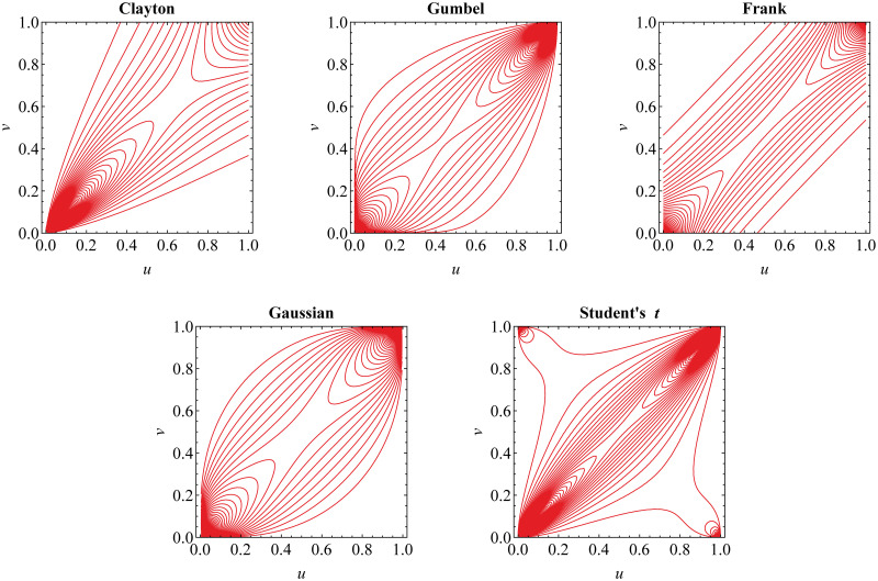
Contour plot for the density of Archimedean and elliptical copulas.
The contours show their different dependence structure for equal Kendall’s τ = 0.6.
Copula selection
For a given risk data set, the challenging task is selecting the best copula which fits well to the data. We may do this by considering several criteria. One of them is Akaike Information Criterion (AIC) introduced by Akaike [39]. Suppose that a copula CU,V(⋅, ⋅;θ) with its corresponding density cU,V(⋅, ⋅;θ) has parameter θ. Based on data

In addition, we employ other criteria by considering empirical version of copula. The empirical copula


Such empirical function is the nonparametric estimate of distribution function,


Vine copula-based modeling
Pair-copula construction method
Suppose that (X, Y, Z) is a dependent risk model consisting of three continuous random variables with joint probability function


Note that


Since


Now, from Eqs (9) and (10), we obtain

This shows that the trivariate copula density cX,Y, Z for (X, Y, Z) model may be constructed from bivariate copula densities: cX,Y, cX,Z, cY,Z|X. In other words, it provides flexible way to determine joint distribution of (X, Y, Z). The first two components cX,Y and cX,Z show dependence of (X, Y) and of (X, Z), respectively, with dependence measure κX,Y and κX,Z. Meanwhile, the component cY,Z|X shows partial dependence of (Y, Z), given X, with partial dependence measure κY,Z|X. Note that the dependence measure of κ may be either Person’s ρ or Kendall’s τ.
Suppose that FX, FY, FZ denote marginal distribution functions of (X, Y, Z). The copula density cX,Y, Z in Eq 11 is basically expressed as


This shows that conditional copula density cY,Z|X is determined through copula CX,Y and CY,Z. From Eqs (12) and (13), copula density cX,Y, Z is completely given by

According to Joe [38], function of CY|X for each copula CX,Y, from Archimedean and elliptical copulas, is given in Table 2. Now, for u = FX(x), v = FY(y) and w = FZ(z), copula density cX,Y, Z is given by


| Copula | Function of CY|X(v|u) |
|---|---|
| Clayton |
 |
| Gumbel |
 |
| Frank | e−θu[(e−θ − 1)(e−θv − 1)−1 + (e−θu − 1)]−1 |
| Gaussian |
 |
| Student’s t |
 |
Note: The function of CY|X is derived for Archimedean and elliptical copulas.
Graph structure and vine (copula)
Suppose that V denotes an empty and finite set. Suppose also that [V]2 = {{v, v′}:v, v′ ∈ V} is a set of all pairs of two unordered elements in V. According to Diestel [43], a graph is a pair (V, E) of sets for some E ⊆ [V]2. The element of V is called node whilst the element of E is an edge. A simple graph
Based on Bedford and Cooke [44, 45] and Kurowicka and Cooke [46],
for all j = 2, 3, …, m − 1,
In short, vine is a collection of nested trees where edge of the jth tree is a node of the (j + 1)th tree.
A vine

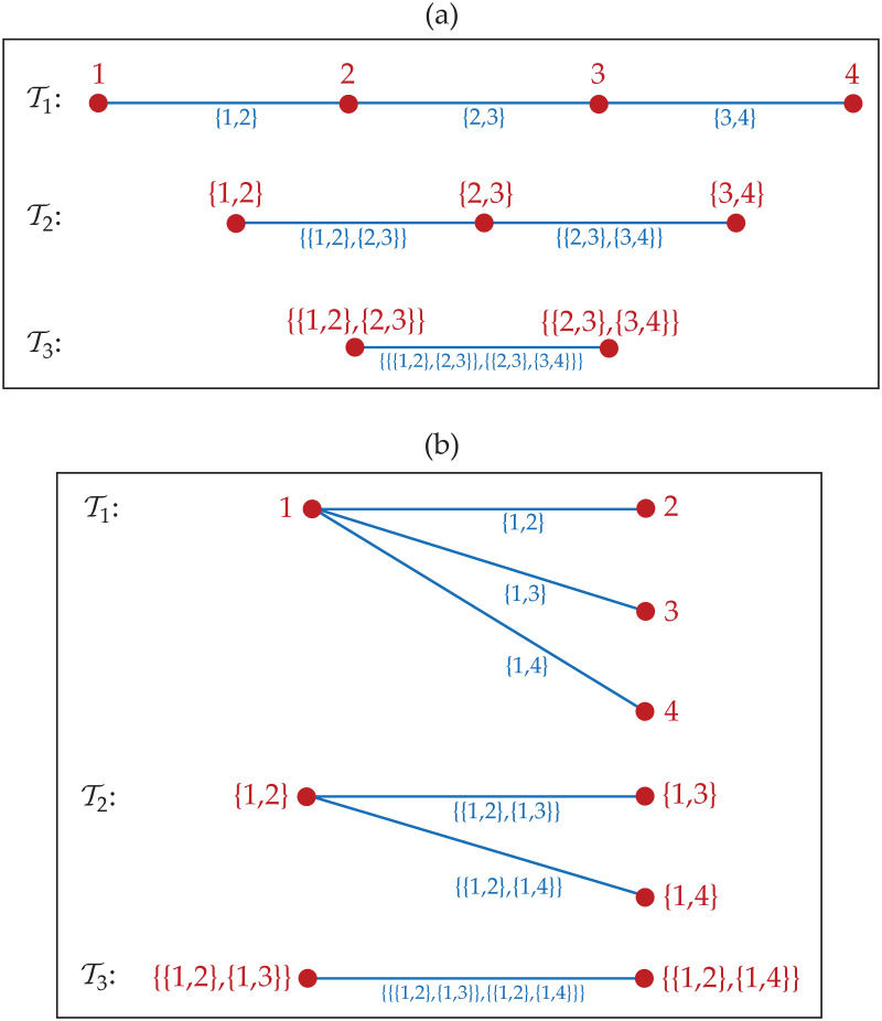
Graph structure of R-vine.
The R-vine is
Now, an R-vine
First, define a complete graph
Forecasting Value-at-Risk (VaR)
Individual VaR forecast
The one-step-ahead VaR forecast is actually a forecast(ing limit) of future risk or return, Xn+1, given previous information up to time n,

Since we use standard Student’s t for innovation distribution and assume GARCH(1,1) for (negative) return model, the conditional distribution of Xn+1, given


Parameter of model, (ωx, δx, βx, νx), may be replaced by its estimate so that we have the estimative one-step-ahead VaR forecast given by

In addition, the estimative ℓ(>1)-step-ahead VaR forecast is as follows

Aggregate VaR forecast
For the case of a portfolio or aggregate risk, we aim to forecast VaR for future aggregate risk of


By employing vine copula, forecasting the one-step-ahead individual VaRs is simultaneously carried out based on the joint distribution of

Then, we may forecast the one-step-ahead aggregate VaR,


This means that the aggVaR forecast above incorporates interactions between different returns by introducing their dependence measures. Note that the estimative aggVaR forecast may be obtained by using the individual estimative VaR forecasts and the estimate of dependence measures.
For perfect (positive) dependence, i.e. κx,y = κx,z = κy,z = 1, it is obvious that the aggVaR forecast is equal to the simple sum of individual VaR forecasts written by

Thus, simplesumVaR may simply be decided as the aggVaR forecast when the worse cases of all of our risks always occur simultaneously, see e.g. Li et at. [49] and Embrechts et al. [2]. In other words, the risks have dependence representation of the form M(u, v, w) = min(u, v, w) which may be called perfect-dependence copula. However, since the dependence measures satisfy |κx,y|, |κx,z|, |κy,z|≤1, we have

This means that the aggVaR forecast in Eq (17) is bounded from above by simplesumVaR in Eq (18). The weaker the dependence among marginal risks, the lower the aggVaR forecast. This is inline with the fact that M(u, v, w) is the upper bound for all classes of copulas, see e.g. Joe [38], including pair-copula which determines the vine copula-based dependence among marginal risks for our portfolio risk.
In addition, it is interesting to investigate diversification benefits of using aggVaR and simplesumVaR. As in Li et at. [49], such diversification benefits may be measured by a so-called diversification coefficient (DC) defined as

From Eq (19), it may be understood that such coefficient is getting higher as the dependence among marginal risks is weaker. This makes the portfolio better diversified.
To find the ℓ-step-ahead aggregate VaR forecast, we consider the vector of ℓ-step-ahead individual VaR forecasts derived simultaneously. We denote it by


The calculation of DC for this aggVaR forecast is analogous to Eq (19) by involving the simple sum of individual VaR forecasts of Eq (20).
Backtesting VaR
After we find the (aggregate) VaR forecast, the assessment of the forecast accuracy is required. It may be carried out through backtesting. From a variety of the backtesting methods, we adopt the methods from Syuhada [34] and Jiménez et al. [20]. We discuss the following methods for the case of
Probability-based backtesting
As stated before, the one-step-ahead VaR forecast is the forecasting limit of future risk, given information of risks in the past. To simply asses the accuracy of VaR forecast, we, therefore, may calculate the probability that the actual future risks do not violate the VaR forecast. It is called coverage probability (CP) defined by

The closer the CP to the confidence level, 1 − α, the more accurate the VaR forecast.
When the sequence of actual future risks,
From the sequence of
Conditional coverage test
The standard test for assessing the accuracy of VaR forecast is the test whether the failure proportion is equal to α. It is basically carried out through binomial test by considering normal approximation of binomial distribution. However, according to Christoffersen [50], the forecast accuracy may be assessed by determining whether the sequence of
The PoF and CCI tests employ likelihood ratio (LR) test statistic. The LR statistic for PoF test is defined by


Backtesting through loss function
It is known that VaR is basically the quantile of (conditional) distribution of the future risk. In addition to the use of inverse of its distribution function, VaR as quantile may be formulated through different approach. Based on Kuan et al. [51],

In this case, the loss function evaluated at our VaR forecast may be relatively compared to that evaluated at VaR forecast obtained from other method as benchmark. They are called quantile losses. The value of their ratio below one means that our forecasting method outperforms the benchmark.
Result and discussion
Daily returns, innovation distribution and marginal risks
The dynamic daily prices and returns for Bitcoin (BTC), Ethereum (ETH) and Litecoin (LTC) for a period of 730 days in 2017-2018 are given in Figs 3 and 4, respectively. The returns follow formula in Eq (1). Whilst the three cryptocurrencies seem to have similar prices behavior, Litecoin has a dramatic increase in day 350 (December 2017) before the decrease in day 400 (February 2018), in comparison to Bitcoin (less dramatic) and Ethereum (gradual increase). In addition, the returns of Litecoin have more high volatility compared to the low and medium volatility as shown in Bitcoin and Ethereum returns, respectively. The property of dynamic volatility significantly appears in all of these returns based on the result of hypothesis test for ARCH effect of Engle [52] in Table 3. This result leads us to assume conditional heteroscedasticity for each of our risk models. Furthermore, the stationarity assumption is also needed based on the result of ADF test in Table 3. In addition, the existence of (inverse) leverage effect may also be considered, especially for Bitcoin whose (negative) return is positively correlated with its squared volatility as visualized in Fig 5. In other words, we also need to assume asymmetric heteroscedastic model in order to capture the feature of asymmetrical volatility. This is in line with assumption in Bouri et al. [25] and Klein et al. [26].


Daily closing prices of cryptocurrencies.
The cryptocurrecy prices are


Negative returns of cryptocurrencies.
The notations of such returns are {Xt}, {Yt} and {Zt} for BTC, ETH and LTC, respectively.

| Test Statistic | BTC | ETH | LTC |
|---|---|---|---|
| ARCH PQ | 105.3 (0.0000) | 120.0 (0.0000) | 48.7 (0.0000) |
| ADF | -717.5 (0.0000) | -709.1 (0.0000) | -717.7 (0.0000) |
Note: The Portmanteau-Q (PQ) test statistic is used to test Engle’s ARCH effect or conditional heteroscedasticity whilst the augmented Dickey–Fuller (ADF) test is for stationarity. The null hypothesis of the tests is rejected due to low p-value (in parentheses) below 5% significance level.


Correlation between (negative) return and its squared volatility.
The significant positive correlation indicates (inverse) leverage effect in the returns data.
We have assumed a GARCH(1,1), as in Eq (2), for each of our risk models. It consists of dynamic volatility and innovation. Table 4 gives the summary of statistics for the estimates of such innovation, defined in Eq (3), for the returns of Bitcoin, Ethereum and Litecoin. It is observed that the high empirical kurtosis leads us to employ heavy-tailed distribution for innovation.

| Statistic | BTC | ETH | LTC |
|---|---|---|---|
| Minimum | -16.8157 | -4.3824 | -7.9936 |
| Maximum | 4.6060 | 4.2687 | 4.9401 |
| Mean | -0.0724 | -0.0615 | -0.0404 |
| Median | -0.0745 | -0.0076 | 0.0229 |
| Std. Deviation | 1.1679 | 0.9342 | 0.9326 |
| Kurtosis | 61.2525 | 6.2055 | 13.987 |
Note: The high kurtosis (above 3) indicates that the innovation is leptokurtic or heavy-tailed.
Furthermore, we visualize the innovation estimates in histogram, Fig 6. Both standard normal and standard Student’s t curves for probability function are fitted, where the estimated degrees of freedom of standard Student’s t are given in Table 5. In fact, it may be observed that standard normal distribution is not appropriate for each innovation. This is also described in Fig 7 for its distribution function. Based on AIC values also given in Table 5, standard Student’s t distribution has lower value of AIC than standard normal distribution. This confirms the appropriateness of standard Student’s t distribution for such innovation, as in Eq (4).


Histogram of innovation estimates.
The histogram for BTC (blue), ETH (green) and LTC (yellow) is fitted to standard normal (black dashed) and standard Student’s t (red) probability functions.


Empirical distribution function of innovations.
The distribution function for BTC (blue), ETH (green) and LTC (yellow) is fitted to standard normal (black dashed) and standard Student’s t (red) distribution functions.

| BTC | ETH | LTC | |
|---|---|---|---|
| Estimate for degrees of freedom | 3.6111 | 2.8916 | 2.8363 |
| AIC for standard Student’s t | 1988.1323 | 1823.1346 | 1745.1279 |
| AIC for standard normal | 2335.3883 | 1977.2438 | 1973.5137 |
Note: The estimate for degrees of freedom is calculated through maximum likelihood method. Lower value of AIC is in boldface.
Based on the assumption above, parameter estimates of GARCH(1,1) model are given in Table 6. By assuming symmetrical volatility, it is observed that the persistence parameters


| Model | Parameter | BTC | ETH | LTC |
|---|---|---|---|---|
| Symmetric | ω | 1.9285 × 10⁻⁵ | 18.432 2 × 10⁻⁵ | 3.1725× 10⁻⁵ |
| δ | 0.0919 | 0.1202 | 0.0758 | |
| β | 0.8337 | 0.6976 | 0.8481 | |
| Asymmetric | ω | 1.9955 × 10⁻⁵ | 18.0567 × 10⁻⁵ | 3.1725 × 10⁻⁵ |
| δ | 0.0892 | 0.1105 | 0.0758 | |
| β | 0.8320 | 0.6995 | 0.8481 | |
| γ | 0.0070 | 0.0214 | 0 |
Note: The estimation is carried out through conditional maximum likelihood method.
Dependence among innovations and the best copula selection
Modeling dependence of (εx;t, εy;t, εz;t) is used to compute and to find joint distribution of
Fig 8 shows scatter plot (three dimension) of innovation estimates


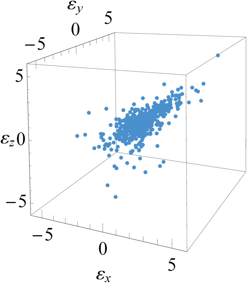
Three dimensional scatter plot of innovation estimates.
The innovation estimates are

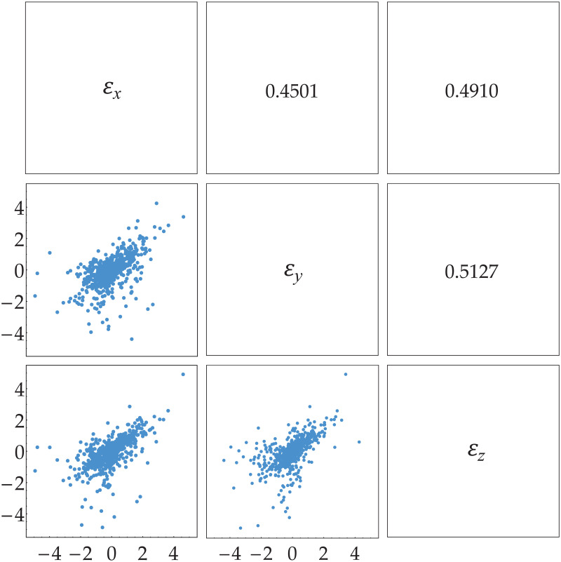
Two dimensional scatter plot of innovation estimates.
The innovation estimates are
Note that the first two bivariate copula densities, respectively, correspond to bivariate copula
According to Aas et al. [11] and Czado et al. [53], copula parameters are estimated through sequential maximum likelihood method as follows. First, the innovation estimates

The transformed data are then used to estimate parameter of copula

The scatter plot of the transformed data {(ut, wt)} and {(vt, wt)} is shown in Fig 10. It may be observed that these transformed data of the estimated innovations show asymmetrical dependence with strong dependence in upper tails. This means that an increase of extremely positive innovation for BTC (or ETH) returns is followed by an increase of that for LTC returns. This empirical fact indicates that Gumbel copula is appropriate for such data. This indication is inline with the result of copula selection based on AIC and goodness-of-fit criteria provided in Table 7. This is because Gumbel copula has the lowest value of AIC and the highest p-value (>0.05) of the goodness-of-fit test for both data {(ut, wt)} and {(vt, wt)}.

| Data | Copula | Estimate (Std. Error) | AIC | GoF (p-value) |
|---|---|---|---|---|
| (a) | Clayton | 0.8202 (0.0680) | -208.3876 | 2.3732 (0.0000) |
| Gumbel | 1.9709 (0.0610) | -513.3633 | 0.0757 (0.2445) | |
| Frank | 5.7798 (0.2920) | -440.1642 | 0.5330 (0.0000) | |
| Gaussian | 0.6244 (0.0190) | -377.3082 | 0.3657 (0.0000) | |
| Student’s t | 0.6894 (0.0210) | -484.0637 | 0.4091 (0.0000) | |
| 3.0795 (0.4210) | ||||
| (b) | Clayton | 0.7725 (0.0660) | -204.8118 | 3.4415 (0.0000) |
| Gumbel | 2.0281 (0.0630) | -531.6440 | 0.1133 (0.0769) | |
| Frank | 6.1585 (0.3040) | -473.6364 | 0.4293 (0.0000) | |
| Gaussian | 0.6339 (0.0180) | -389.5267 | 0.6240 (0.0000) | |
| Student’s t | 0.7049 (0.0200) | -486.3833 | 0.5506 (0.0000) | |
| 3.0055 (0.3880) |
Note: The estimation for parameter of Archimedean and elliptical copulas is carried out through maximum likelihood method whilst the goodness-of-fit test uses Cramér–von Mises statistic. The lowest value of AIC and the highest p-value for certain data are in boldface.

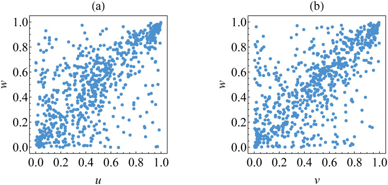
Transformed data for determining the best copulas for the first tree graph.
The data are (a) {(ut, wt)} and (b) {(vt, wt)}.
In addition, graphical approach visualized in Fig 11 explains that Kendall’s distribution function (and the corresponding function of λ) derived from Gumbel copula seem to be close enough to the empirical Kendall’s distribution function defined in Eq (7) (and the empirical function of λn defined in Eq (8)). This means that Gumbel copula fits well to the upper-tail dependent data {(ut, wt)} and {(vt, wt)}.

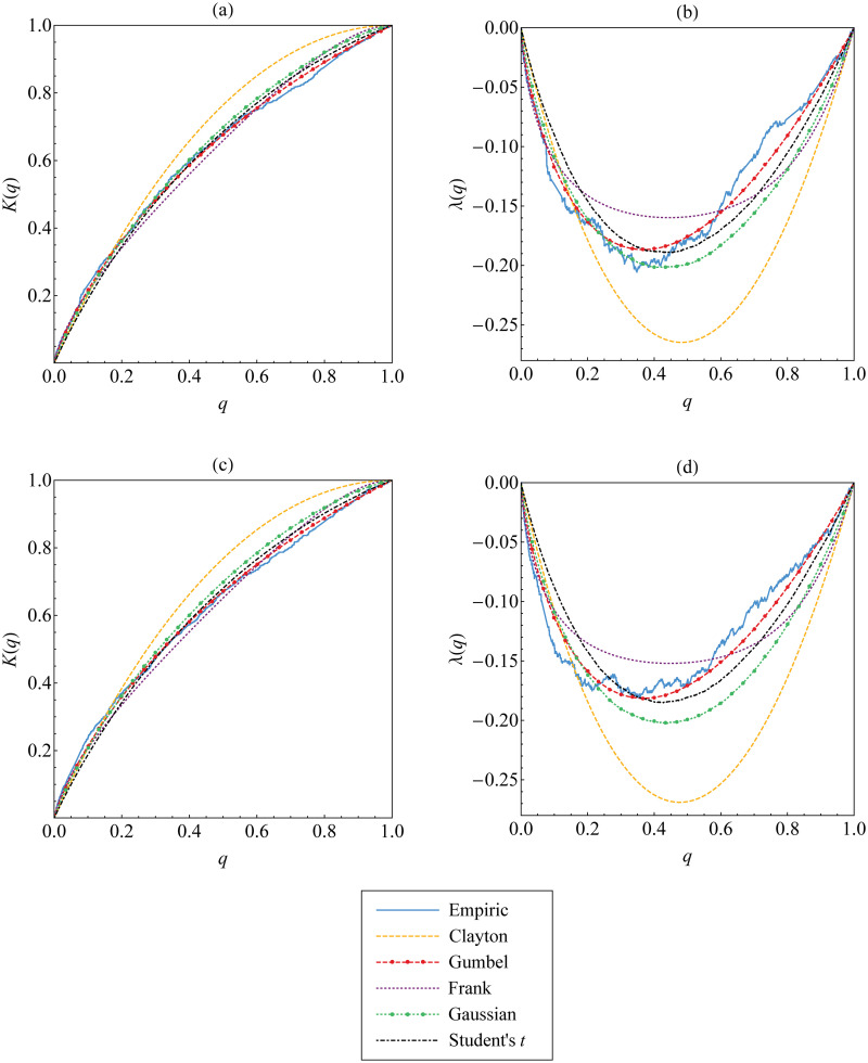
The best copula selection for the first tree graph based on Kendall’s distribution function and the corresponding function of λ.
Such functions for Archimedean and elliptical copulas are compared and fitted to those for empirical copula of the data (a-b) {(ut, wt)} and (c-d) {(vt, wt)}.
From the result above, Gumbel copula is the best fitting copula for

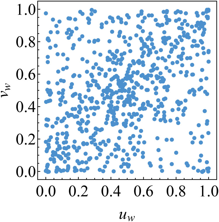
Transformed data for determining the best copula for the second tree graph.
The data are {(uw;t, vw;t)} with

| Copula | Estimate (Std. Error) | AIC | GoF (p-value) |
|---|---|---|---|
| Clayton | 0.2376 (0.0920) | -43.6005 | 0.9125 (0.0000) |
| Gumbel | 1.2364 (0.0350) | -79.4680 | 0.2910 (0.0041) |
| Frank | 2.4035 (0.2560) | -85.3951 | 0.1178 (0.0659) |
| Gaussian | 0.2616 (0.0310) | -58.7777 | 0.1691 (0.1644) |
| Student’s t | 0.3221 (0.0370) | -107.0723 | 0.0985 (0.4384) |
| 5.5976 (1.0060) |
Note: The estimation for parameter of Archimedean and elliptical copulas is carried out through maximum likelihood method whilst the goodness-of-fit test uses Cramér–von Mises statistic. The lowest value of AIC and the highest p-value are in boldface.

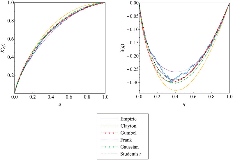
The best copula selection for the second tree graph based on Kendall’s distribution function and the corresponding function of λ.
Such functions for Archimedean and elliptical copulas are compared and fitted to those for empirical copula of the data {(uw;t, vw;t)}.
By merging the results above, the best dependence model for (εx;t, εy;t, εz;t) based on the data of innovation estimates


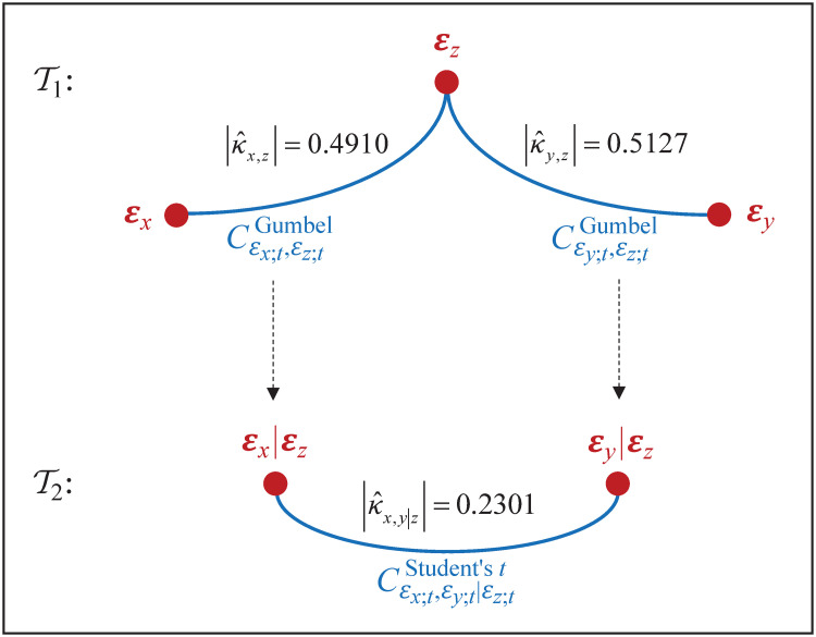
Representation of joint distribution for innovations.
The joint distribution for

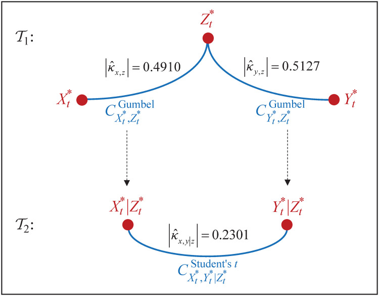
Representation of joint distribution for returns.
The joint distribution for
VaR forecast
Now, the one-step-ahead VaR forecasts for Bitcoin, Ethereum and Litecoin returns based on (a)symmetric GARCH(1,1) model are provided in Table 9. Such VaR forecasts are calculated at 95%, 97% and 99% confidence levels (CLs) under two assumptions: (i) perfect dependence, as benchmark, and (ii) vine copula-based dependence among different returns. For the former assumption, we simulate perfectly dependent innovations to calculate the previous returns and volatility and, hence, to find the individual VaR forecasts. This procedure is similarly applied for the latter assumption for which the innovations are simulated through vine copula we have previously determined. Note that the individual VaR forecasts are found simultaneously by Eq (16) for one day only.

| Model | Currency | CL | VaR | CP | AE | CC (p-value) | QL (Ratio) |
|---|---|---|---|---|---|---|---|
| Under perfect dependence assumption | |||||||
| Symmetric | BTC | 95% | 0.0237 | 95.24% | 0.9517 | 0.3417 (0.8429) | 0.00199 |
| 97% | 0.0297 | 97.52% | 0.8276 | 4.7255 (0.0942) | 0.00149 | ||
| 99% | 0.0456 | 99.24% | 0.7586 | 4.2226 (0.1211) | 0.00084 | ||
| ETH | 95% | 0.0462 | 96.69% | 0.6624 | 12.6247 (0.0018) | 0.00365 | |
| 97% | 0.0617 | 98.27% | 0.5751 | 12.7249 (0.0017) | 0.00280 | ||
| 99% | 0.1103 | 99.45% | 0.5521 | 8.0716 (0.0177) | 0.00159 | ||
| LTC | 95% | 0.0285 | 96.41% | 0.7177 | 8.7266 (0.0127) | 0.00254 | |
| 97% | 0.0380 | 98.27% | 0.5751 | 12.7249 (0.0017) | 0.00202 | ||
| 99% | 0.0680 | 99.38% | 0.6211 | 6.5150 (0.0385) | 0.00127 | ||
| Asymmetric | BTC | 95% | 0.0238 | 95.24% | 0.9517 | 0.3417 (0.8429) | 0.00200 |
| 97% | 0.0303 | 97.52% | 0.8276 | 4.7255 (0.0942) | 0.00149 | ||
| 99% | 0.0466 | 99.24% | 0.7586 | 4.2226 (0.1211) | 0.00084 | ||
| ETH | 95% | 0.0459 | 96.55% | 0.6901 | 10.5727 (0.0051) | 0.00362 | |
| 97% | 0.0613 | 98.27% | 0.5751 | 12.7249 (0.0017) | 0.00278 | ||
| 99% | 0.1096 | 99.45% | 0.5521 | 8.0716 (0.0177) | 0.00157 | ||
| LTC | 95% | 0.0285 | 96.41% | 0.7177 | 8.7266 (0.0127) | 0.00254 | |
| 97% | 0.0380 | 98.27% | 0.6671 | 12.7249 (0.0017) | 0.00202 | ||
| 99% | 0.0680 | 99.38% | 0.6211 | 6.5150 (0.0385) | 0.00127 | ||
| Under vine copula-based dependence assumption | |||||||
| Symmetric | BTC | 95% | 0.0230 | 94.98% | 1.0041 | 0.1441 (0.9305) | 0.00192 (0.9640) |
| 97% | 0.0288 | 96.97% | 1.0087 | 0.0995 (0.9515) | 0.00141 (0.9493) | ||
| 99% | 0.0443 | 98.97% | 1.0316 | 0.3272 (0.8491) | 0.00068 (0.8107) | ||
| ETH | 95% | 0.0458 | 95.59% | 0.8822 | 1.1211 (0.5709) | 0.00362 (0.9910) | |
| 97% | 0.0611 | 97.79% | 0.7351 | 3.5742 (0.1674) | 0.00271 (0.9657) | ||
| 99% | 0.1091 | 99.31% | 0.6892 | 1.7278 (0.4215) | 0.00135 (0.8469) | ||
| LTC | 95% | 0.0276 | 96.01% | 0.7989 | 3.3590 (0.1865) | 0.00219 (0.8621) | |
| 97% | 0.0369 | 98.07% | 0.6428 | 6.8704 (0.0322) | 0.00165 (0.8154) | ||
| 99% | 0.0659 | 99.17% | 0.8264 | 3.4289 (0.1801) | 0.00083 (0.6492) | ||
| Asymmetric | BTC | 95% | 0.0233 | 94.98% | 1.0041 | 0.1441 (0.9305) | 0.00194 (0.9686) |
| 97% | 0.0292 | 96.97% | 1.0087 | 0.0995 (0.9515) | 0.00143 (0.9564) | ||
| 99% | 0.0449 | 98.83% | 1.1692 | 0.8009 (0.6700) | 0.00069 (0.8202) | ||
| ETH | 95% | 0.0457 | 94.70% | 1.0599 | 1.7564 (0.4155) | 0.00360 (0.9947) | |
| 97% | 0.0610 | 97.25% | 0.9176 | 2.9389 (0.2300) | 0.00269 (0.9698) | ||
| 99% | 0.1090 | 99.24% | 0.7571 | 2.5563 (0.2786) | 0.00133 (0.8505) | ||
| LTC | 95% | 0.0276 | 96.01% | 0.7989 | 3.3590 (0.1865) | 0.00219 (0.8621) | |
| 97% | 0.0369 | 98.07% | 0.6428 | 6.8704 (0.0322) | 0.00165 (0.8154) | ||
| 99% | 0.0659 | 99.17% | 0.8264 | 3.4289 (0.1801) | 0.00083 (0.6492) | ||
Note: The one-step-ahead individual VaR forecasts for BTC, ETH and LTC returns are found simultaneously for one day only based on simulated innovations through perfect-dependence copula (for the first assumption) and through vine copula (for the second assumption). The resulted p-value of CC test in boldface is higher than 5% significance level. Meanwhile, the QL ratio in boldface is below one, which means that vine copula-based forecasting procedure performs better.
The forecast accuracy under two assumptions above is assessed and compared through several backtesting methods adopted from Syuhada [34] and Jiménez et al. [20]. These methods include coverage probability (CP), actual over expected (AE) ratio, conditional coverage (CC) test and quantile loss (QL) ratio.
We find that the VaR forecasts for returns by assuming vine copula-based dependence have higher forecast accuracy. This is because the CP for these VaR forecasts are closer to the corresponding CL and their AE ratio are closer to one. Furthermore, this assumption successfully passes the CC test since the resulted p-value is higher than 5% significance level, except for Litecoin at the 97% CL with p-value 0.0322. The choice of significance level may be relaxed to 1% so that the CC test for Litecoin at such CL is also passed. Such results are obtained based on both symmetric and asymmetric GARCH(1,1) models. These show the positive impact of vine copula-based dependence on the VaR forecasts. These are confirmed from the low value of all QL ratios below one. As the CL increases, the QL ratio is getting lower. Meanwhile, the consideration of using asymmetric model do not give better impact on the VaR forecasts. This is because the VaR forecasts derived from both symmetric and asymmetric models do not obviously differ, but the asymmetric model provides higher value of QL ratio.
As mentioned before, we have used the empirical data from 1-1-17 till 31-12-18. Now, we compare the VaR forecasts for several steps/days to the empirical data from 1-1-19 till 31-12-19 as visualized in Fig 16. The comparison is made based on (a)symmetric GARCH(1,1) model where the VaR forecasts are calculated simultaneously by Eq (20) through vine copula.

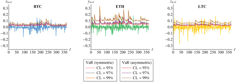
VaR forecasts of marginal risks for several steps/days.
The forecasts are derived at 95%, 97% and 99% confidence levels (CLs) based on symmetric (solid line) and asymmetric (dashed line) GARCH(1,1) models for Bitcoin (BTC), Ethereum (ETH) and Litecoin (LTC) through vine copula. They are also compared to the real data.
According to the result in Table 9, we now provide, in Table 10, the one-step-ahead forecast of portfolio risk by using aggregate VaR (aggVaR) through vine copula in comparison to the simple sum of individual VaRs (simplesumVaR), as the benchmark, for one day only. Their forecast accuracy is compared in terms of CP, AE ratio, CC test and QL ratio. We may observe that the aggVaR forecast is lower in value with better accuracy at each CL. The CP as well as AE ratio are closer to the target and the CC test is successfully passed at 5% significance level. Meanwhile, in calculating simplesumVaR, the rejection of null hypothesis of the CC test is only at low level of significance, e.g. 1%, due to the low p-value. Furthermore, the QL ratio between aggVaR and simplesumVaR is below one and getting lower as the CL increases. These show that calculating simplesumVaR is too conservative and overestimates the portfolio risk. In other words, vine copula-based forecasting procedure outperforms perfect dependence assumption. The use of vine copula also makes the portfolio diversified, with diversification coefficient (DC) about 18%. Considering diversification typically provides a stable portfolio since overall risk of the portfolio is properly reduced and, hence, risk allocation is allowed. However, as shown in Table 10, the DC is getting lower as the CL increases. This means that the higher the CL, the less stable the portfolio. The results under symmetric and asymmetric GARCH(1,1) models are in line. However, the asymmetric one performs worse with higher value of the QL ratio although the resulted DC is higher.

| Model | CL | VaR Forecast | DC% | CP | AE | CC (p-value) | QL (Ratio) | |
|---|---|---|---|---|---|---|---|---|
| Symmetric | 95% | simplesum | 0.0964 | 17.95 | 96.27% | 0.7453 | 7.0780 (0.0290) | 0.00812 |
| aggVaR | 0.0791 | 94.73% | 1.0548 | 1.1926 (0.5508) | 0.00719 (0.8856) | |||
| 97% | simplesum | 0.1267 | 17.80 | 97.93% | 0.6901 | 6.8669 (0.0323) | 0.00627 | |
| aggVaR | 0.1042 | 97.15% | 0.9484 | 0.1473 (0.9290) | 0.00534 (0.8517) | |||
| 99% | simplesum | 0.2194 | 17.42 | 99.38% | 0.6211 | 6.5150 (0.0385) | 0.00368 | |
| aggVaR | 0.1812 | 98.89% | 1.1103 | 2.0685 (0.3555) | 0.00265 (0.7193) | |||
| Asymmetric | 95% | simplesum | 0.0966 | 17.99 | 96.27% | 0.7453 | 7.0780 (0.0290) | 0.00811 |
| aggVaR | 0.0792 | 94.73% | 1.0548 | 1.1926 (0.5508) | 0.00719 (0.8872) | |||
| 97% | simplesum | 0.1271 | 17.84 | 97.93% | 0.6901 | 6.8669 (0.0323) | 0.00625 | |
| aggVaR | 0.1044 | 97.15% | 0.9484 | 0.1473 (0.9290) | 0.00533 (0.8534) | |||
| 99% | simplesum | 0.2198 | 17.46 | 99.38% | 0.6211 | 6.5150 (0.0385) | 0.00366 | |
| aggVaR | 0.1815 | 98.89% | 1.1103 | 2.0685 (0.3555) | 0.00264 (0.7207) | |||
Note: The aggregate VaR forecast is calculated for one day only through vine copula and is compared to the simple sum of individual VaR forecasts. The diversification coefficient is also calculated. The resulted p-value of CC test in boldface is higher than 5% significance level whilst the QL ratio in boldface is below one.
In addition, we calculate the aggVaR forecasts for several steps/days. Such forecasts are visualized in Fig 17. This figure also provides their comparison to the simplesumVaR and the real data of aggregated returns from 1-1-19 till 31-12-19. Meanwhile, the corresponding DCs are displayed in Fig 18.


VaR forecasts of portfolio risk for several steps/days.
The aggVaR forecasts are calculated at 95%, 97% and 99% confidence levels (CLs) based on symmetric (solid line) and asymmetric (dashed line) models through vine copula. They are compared to the simplesumVaR (purple) and to the real data (blue).

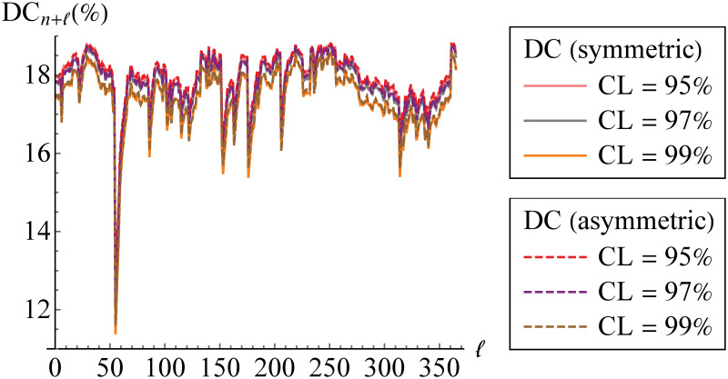
Diversification coefficients of aggregate VaR forecasts.
The diversification coefficients (DCs) are calculated at 95%, 97% and 99% confidence levels (CLs) based on symmetric (solid line) and asymmetric (dashed line) models through vine copula.
Conclusion
Model for dependent risks that form a portfolio risk has been constructed. Through vine copula, their marginal risks assumed to follow GARCH(1,1) model are coupled with complete representation through graph structure. This approach provides high flexible pair-copula model since it is able to capture dependence structure of all possible pairs of risks by using different bivariate copulas with the best criterion. As we hope, applying this dependence model to forecast VaR for Bitcoin, Ethereum and Litecoin returns provides good forecast accuracy. Furthermore, the resulted portfolio VaR forecast is low in value with high accuracy instead of simply summing the individual VaR forecasts under perfect dependence assumption. As a consequence, the portfolio is well diversified which means that its overall risk is well managed and reduced. The results under consideration of both symmetrical volatility and asymmetrical volatility in the marginal model are in line. However, the asymmetric model does not perform better although it makes the portfolio more diversified.
For further research, modeling dependence may be carried out for higher-dimensional risk data due to the increasing number of risks in the cryptocurrency market or other markets nowadays. Furthermore, the marginal risk model may be extended to another observable volatility models of GARCH. The use of latent volatility model of Stochastic Volatility Autoregressive (SVAR), see e.g. Han et al. [54] and Syuhada [34], perhaps gives more interesting results. This is due to volatility shock that appears in volatility process. As for risk measure forecast, it is important to consider (i) expected-based risk measure, namely Expected Shortfall or Tail-VaR, and (ii) expectile-based risk measure of EVaR [51]. Whilst the former (VaR) is more probability-based risk measure, the latter (ES/TVaR, EVaR) takes the magnitude of losses into account.
Acknowledgements
We are grateful to the academic editor’s and reviewers’ comments, careful reading and numerous suggestions that greatly improved this paper.
References
1
2
3
4
5
6
7
8
9
10
11
12
13
14
15
16
17
18
19
20
21
22
23
24
25
26
27
28
29
30
31
32
33
34
35
36
37
38
39
40
41
42
43
44
45
46
47
48
49
50
51
52
53
54
 Modeling risk dependence and portfolio VaR forecast through vine copula for cryptocurrencies
