Data

We used 13 of the 15 cohorts used in [15]. We designate Cohorts MAINZ (n = 200), STAM (n = 856) and UPSA (n = 289) as test cohorts (this is the same as in [15]). We use the remaining 10 cohorts as training cohorts, for a total of 4546 samples with 9461 genes. All the gene expressions in all the cohorts are normalized and have a distribution of N(0, 1). When driving our selection by classification accuracy, we use 20% as a validation set for determining the final selected set of genes. When driving our selection by log rank performance, we combine 50% of the test cohorts to serve as a validation set. The other half serves as test data for the log rank performance. We now describe, in detail, the three stages of our selection process:

Wilcoxon rank-sum (WRS) filtering.

Iterative logistic regression.

Select the best set of genes according to the validation set—first using normalized expression and second, based on relative expression.

WRS filtering

Our first step is to run a WRS test [16, 17] as a filter method. The selection of the genes in this step is independent of any machine learning algorithm. We filter out genes that are not differentially expressed with respect to Cluster B vs. Not Cluster B, as defined in [15]. We use p-value = 0.1 as our threshold and each gene with a WRS p-value > 0.1 is filtered out. After the WRS filtering, we are left with 6557 genes, out of the initial 9461 genes. This point represents a False Discovery Rate (FDR) [18] of 0.14.

Iterative lasso logistic regression

Iterative approaches, such as Orthogonal Matching Pursuit (OMP—[19]), have proven to be efficient in feature selection processes. Using the OMP approach, we construct the set of features iteratively, working with z-score normalized feature values. Each iteration consists of running a regression algorithm and selecting the feature with the highest weight. The process is initialized with the target vector $$ \overrightarrow{y}$$ and, in each iteration, the target is updated to the residual. Since the features are normalized, the weights of the solution vector are associated with the impact of each feature on the predicted variable. The greater the weight (absolute value), the greater the effect on the prediction value. We use this property to drive an iterative lasso backward selection algorithm. We note that applying forward selection in our data yielded far inferior results and the backward approach certainly led to better performance. Specifically, forward selection produced a validation accuracy of 0.8 while our iterative lasso backward selection algorithm generated a validation accuracy of 0.91.

Another approach is the Relaxed Lasso [20], where the lasso regression is executed twice with different regularization factors. [20] demonstrates, using theoretical and numerical evidence, that Relaxed Lasso produces sparser models with equal or lower prediction losses than the regular lasso estimator for high-dimensional data.

Our approach is an iterative one that starts with all features and rejects features as we move through a while loop. In each iteration we run a logistic regression penalized by lasso (λ = 1) to calculate the weight for each gene. Then, we remove genes with low weight (absolute value). In the first iterations, we remove 10% of the genes with the lowest weights (absolute value). From 900 genes downwards, we remove only one gene in each iteration. The pseudocode is given in Algorithm 1.

Algorithm 1: Pseudocode of the algorithm we use for selecting an efficient set of genes, where LR(D, Ω) is the logistic regression algorithm (lasso in our case) and $$ nnz\left(\overrightarrow{w}\right)$$ is the number of non-zero elements in $$ \overrightarrow{w}$$. The function argsort sorts the indices of an array according to the values it contains.

Iterative logistic regression gene set selection

input: Normalized gene expression dataset—D

output: Sparse gene expression dataset

initialization

Ω = {set of all genes}

$$ \overrightarrow{w}\ne 0$$

while $$ nnz\left(\overrightarrow{w}\right)>900$$ do

 $$ \overrightarrow{w}=LR(D,\Omega )$$

 // find the indices of 10% smallest absolute values

 sorted_index_w = argsort(|w|)

 10%_index = 0.1 × size(w)

 smallest_set = sorted_index_w[0:10%_index]

 Ω = Ω−smallest_set

end

while $$ nnz\left(\overrightarrow{w}\right)>50$$ do

 $$ \overrightarrow{w}=LR(D,\Omega )$$

 smallest_w_index = argmin(|w|)

 Ω = Ω−smallest_w_index

end

return Ω

Selection based on classification accuracy

We combine our iterative approach with a training/validation split. In each iteration, we calculate the validation accuracy. Classifiers are trained with a three-way loss function for clusters A, B and C. For the validation we evaluate Cluster B vs. Not Cluster B. We select the best performing set of genes. This process yields Point A in Fig 1. The set of genes thus obtained is called Γ_A.

Fig 1

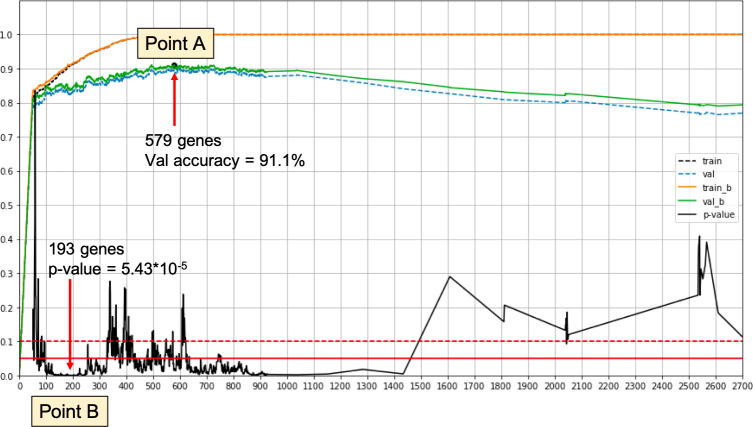
Overview illustration of the gene selection process.

Point A—Best validation accuracy for the classification driven process. Point B—Best log rank p-value on a validation set. The signature of Point B achieves log rank p-value < 2 × 10⁻⁴ and log rank p-value < 2 × 10⁻³ when using only relative expression values.

Selection based on log rank performance

In this process we incorporate the log rank test into the training phase. We take the test cohorts with 1300 samples and split them into validation and test sets. We use the new validation set in the iterative process to evaluate the performance after each iteration. In each iteration we predict the label of all validation samples and then conduct a log rank test comparing the samples called Cluster B to those called Not Cluster B. We choose the set of features with the smallest log rank p-value. This process yields Point B in Fig 1. The set of genes thus obtained is called Γ_B.

A signature based on relative expression

In practice, results derived from the normalized data are not directly useful in working with new samples. When diagnosing a single patient, no normalization context can be assumed—beyond that which is internal to the patient’s sample. To enable practical use of the genes in Γ_B, we trained a new classifier based on their relative expression as derived from the raw data that underlies the samples in our training set. The idea is that the relative expression levels of these genes can be computed in the context of any signature sample, without the need to normalize it back to the context of the training cohorts. For this purpose, consider the raw expression data instance E(g, d) measured for every gene g and a single sample d. We define a relative expression value Q(g, d) for every g ∈ Γ_B and every training sample d. First we sort E(g, d) to get the ranks 1 ≤ R(g, d) ≤ N = |Γ_B| (= 193). Now define:

In other words, we map every gene to its relative decile within the set Γ_B, in the context of sample d.

We now train a Naive Bayes classifier, based on the features Q(g, d), to classify the samples into two prognostic subclasses: GPx = Not_Cluster_B and BPx = Cluster_B. To classify a new sample (which has not been seen in the training process), we just transform all gene expression levels there, for all g ∈ Γ_B, to relative levels (rank deciles) as above and execute the trained classifier. Note that 10 is obviously a hyperparameter of this process.

Kaplan Meier curves

The Kaplan Meier curves in this paper were generated using the Python library lifelines. They include the 0.95 confidence envelope and an indication of the Q3 level of survival for each class with corresponding colors.

Selected efficient signatures

The two feature selection approaches described in the Methods section resulted in two gene sets with the best observed performance:

579 genes for the classification accuracy driven approach; designated as Point A in Fig 1.

193 genes for the log rank performance driven approach; designated as Point B in Fig 1.

Note that when using different training validation set splits, we may get different results. This point is addressed below. An overview of the selection process, as run on our data, is depicted in Fig 1.

Improved Cluster B classification with 579 genes

We compared our results to [15]. As shown in Table 1, we improved the classifier recall and the AUC. We also improved the log rank p-value slightly. We note that we also achieved a modest advance in the number of genes that support the signature.

Table 1

Performance overview—Point A.

	This work	Tekpli et al.
# genes	579	658
Cluster B recall	0.89	0.69
AUC	95.4%	85.8%
Log rank p-value	0.00018	0.00027

Working with these 579 signature genes that we found, we classified the test samples and applied log-rank statistical analysis on the results of the classification. We observe, as in [15], a prognostic disadvantage to the samples called Cluster B (see Fig 2).

Fig 2

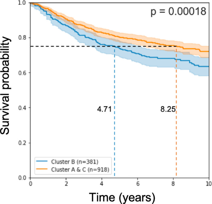
Kaplan Meier curve and log rank p-value on the test cohorts.

The model used 579 genes for learning.

Improved prognostic signature with 193 genes

Reducing the number of selected genes reduces the classifier’s performance as well, as we can see in Table 2. The procedure of feature selection for better prognosis is a new task and will be further addressed below. Although the classifier’s performance decreased, the log rank p-value stayed the same and the number of selected genes dropped to 193.

Table 2

Performance overview—Point B.

	This work	Tekpli et al.
# genes	193	658
Cluster B recall	0.71	0.69
AUC	89.4%	85.8%
Log rank p-value	0.00017	0.00027

Working with these 193 signature genes that we found, we classified the half of the test samples we left for testing and applied log-rank statistical analysis on the results of the classification. As in approach 1 above, the prognostic disadvantage to the samples called Cluster B remains significant (see Fig 3).

Fig 3

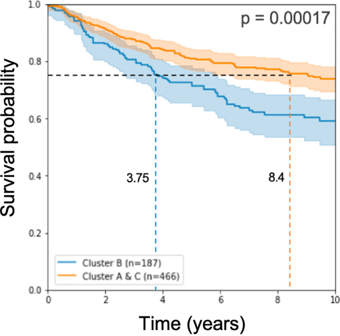
Kaplan Meier curve and log rank p-value on half of the test cohorts.

The model used 193 genes for learning.

A signature based on relative expression yields accurate prognostic predictions

As described in the Methods section, we applied a Naive Bayes approach to classify test patients according to their predicted prognosis: GPx (good prognosis) and BPx (bad prognosis). Survival analysis results in a log rank p-value of 10⁻³ when computed for n = 653 test samples (see Fig 4).

Fig 4

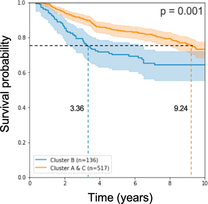
Kaplan Meier curve and log rank p-value on half of the test cohorts.

The model used expression rank values from 193 genes for learning.

Trained classifier results are associated with tumor infiltrating lymphocytes levels

We further examined our classification results on the training set, using the 193 gene set (Point B). We checked that the association between the clusters and the lymphocyte infiltration did not break. As we can see in Fig 5, the lymphocyte infiltration is increasing when moving from Cluster A to Cluster B to Cluster C. We also tested the significance of the classes using the Kruskal–Wallis test, as in [15], and got a value of 4 × 10⁻²⁹⁶ & 7 × 10⁻¹⁸ for the Metabric and MicMa cohorts, respectively. These results are similar to these of [15].

Fig 5

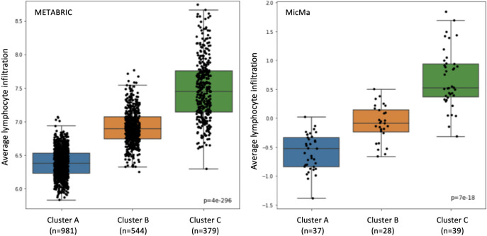
Lymphoid score differences.

Lymphoid scores are represented in box-plots according to the training predictions with the selected 193 genes. On the left is the Metabric cohort and on the right, the MicMa cohort.

Enrichment analysis

We used the GOrilla (Gene Ontology enRIchment anaLysis and visuaLizAtion) [21, 22] tool to examine statistical enrichment of GO (Gene Ontology) annotations. As shown in Fig 6, our selected set of 193 genes is significantly enriched with immune system genes.

Fig 6

Gene Ontology biological processes statistically enriched in the selected 193 genes, using GOrilla [21, 22].

Color intensity represents the statistical significance of the enrichment.

Characteristics of BPx

To understand more deeply our findings, we examined the BPx class.

First, we analyzed the composition of BPx, in terms of known breast cancer subtypes and other patient characteristics. The results are described in S1 Fig in S1 Text. The properties analyzed include age, tumor grade, tumor stage, laterality, lymph node metastasis number, ER status and others. In summary, we cannot reject the no difference null hypothesis for any subset of the tested properties at FDR = 0.05. The composition of BPx, in terms of PAM50 subtypes, is further addressed below.

Second, we compared BPx to [15]’s Immune Cluster B (CB) in the combined cohort of 4546 patients. We observed 447 patients in the symmetric difference CBΔBPx. Of these, we observed 268 patients in CB\BPx and 179 patients in BPx\CB. Ranking genes according to differential expressions between these two sets (using WRS), we found 21 genes that have a significantly lower expression in CB at FDR = 0.05 (genes and p-values reported in Differentially expressed genes CB vs. BPx in S1 Text).

Finally, in Metabric [23] the authors also report mutation status for 173 genes. We found (using a hypergeometric test) that mutations in GATA3 have a lower frequency in the BPx class at FDR = 0.05, which is depleted at p-value = 0.003 (52/544 in BPx, 194/1360 in GPx). GATA3 is one of three genes (the other two are TP53 and PIK3CA) that were reported to have somatic mutations at more than 10% incidence across all breast cancers [24]. There is disagreement, however, about the role of GATA3, with some studies suggesting that GATA3 functionality acts to inhibit, and other studies suggesting that it acts to promote, the development, growth, and/or spread of breast cancer. The second most significant gene with mutations observed, in terms of differences between BPx and GPx, is MAP3K1 (50/544 in BPx and 173/1360 in GPx, p-value = 0.017). Both GATA3 and MAP3K1 are known to have important roles in breast cancer [24–27]. In the Metabric cohort there were ten patients observed with somatic mutations in both GATA3 and MAP3K1. All ten patients were BPx (hypergeometric p-value = 3.41 × 10⁻⁶, N = 1904, B = 10, n = 544, b = 10). Moreover, nine of them were LumA and Her2+ BPx patients (hypergeometric p-value = 1 × 10⁻⁷, N = 1904, B = 10, n = 253, b = 9).

Limitations and future directions

In this work we applied feature selection techniques to improve a prognostic immune related signature previously suggested in [15]. We obtained a classifier that uses 193 genes and yields a log rank p-value < 2 × 10⁻⁴ on test data. As we noted above, using different training validation set splits may yield different results. We ran the process with ten different splits (see Table 3). We observed 11 genes in the intersection of the 10 sets obtained in this manner. Observing such an intersection at random, under a uniform/independent null model, is highly significant (p-value < 10⁻¹⁰⁰).

Table 3

Results for ten different splits.

	# genes	Validation accuracy	Log-rank p-value
1	91	93.4%	0.001
2	192	90.1%	0.0007
3	53	93.5%	0.0004
4	134	93.0%	0.04
5	109	93.4%	0.001
6	52	91.2%	0.004
7	193	93.1%	0.05
8	64	93.5%	0.02
9	68	93.0%	0.004
10	88	91.3%	0.003

It is important to note that the survival data used in this paper is overall survival data. In particular, our findings do not imply a signature that would be indicative of the response to any particular therapy.

To develop classifiers driven by survival data, one needs to use validation data for which feature values and survival information are available. The task of optimizing a classifier using quantitative features requires, and merits, much deeper investigation, in a broader context. The methods described in [28] address a similar question in the context of class discovery driven by a one-dimensional quantitative feature. That work does not, however, address survival to any extent.

It is also interesting to examine the classification obtained by the Naive Bayes classifier on the test samples. Fig 7 depicts the distribution of PAM50 subtypes in the two classes, BPx and GPx. Note that although the PAM50 partition is not independent of the class (χ² p-value = 0.002), neither prognostic subset is significantly aligned with a PAM50 subtype.

Fig 7

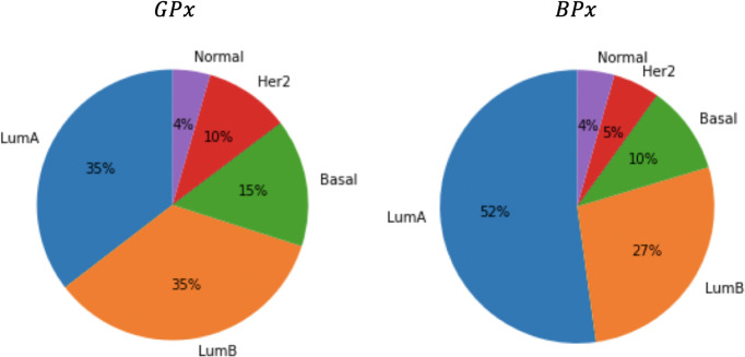
Pie charts of the PAM50 typing in the two different prognostic classes: GPx and BPx.

One obvious future research direction is the development of even more efficient prognostic signatures for breast cancer. A related task would be to include other types of measurement (copy number measurement, methylation, miRNA profiling etc.) to improve the predictive power.

Can the combination of Tumor Infiltrating Lymphocyte (TIL) levels with the expression signature lead to an even more significant prognostic indication? According to [15] and to other studies, TIL levels can be important in this context. An extension of our study would be to see how we can combine the expression-based immune signature with information about TIL levels.

The development of expression-based signatures calls for using sparse feature selection techniques. The literature addresses sparse feature selection in a variety of machine learning contexts. Questions related to which of these methods work for survival analysis is a topic for further research. In this study we explored several heuristic approaches. Some of them can be further generalized. Moreover, the direct use of survival data to drive feature selection and the development of methods for doing so will require further research and development.