Issues with Straightforward Application of PICs

Dunn et al. (2018) have made a relevant argument that the ortholog conjecture test should be done in a phylogenetic framework, as closely related species or genes tend to share more similar traits. They applied PIC to 8,520 time-calibrated trees (table 1) and reported evidence against the ortholog conjecture for tissue specificity $$ \tau \mathrm{ }$$(median: PIC_speciation = 0.0072, PIC_duplication = 0.0051, one-sided Wilcoxon test P = 1). Yet, the same data supported the ortholog conjecture when analyzed by pairwise comparisons both in Kryuchkova-Mostacci and Robinson-Rechavi (2016) and in the re-analysis by Dunn et al. (2018). To understand the incongruence between PIC and pairwise comparisons, they performed simulations of $$ \tau $$ on their trees under the ortholog conjecture and under a null of uniform BM. Both methods should be able to distinguish the null from the ortholog conjecture for diverse trees (supplementary fig. S1, Supplementary Material online). Under the simulations of Dunn et al. (2018), pairwise comparisons could not distinguish the two scenarios, whereas the PIC could. As their results on empirical data resembled those on the null simulation, they questioned both the use of pairwise comparisons and the support for the ortholog conjecture from tissue specificity data.

Table 1.

Information on Different Tree Sets, Number of Internal Node Events, and Node Ages Used in This Reanalysis.

Data Sets	Number of Trees	Number of Speciation Events	Number of Duplication Events	Number of NA Events	Maximum Speciation Node Age (My)	Maximum Duplication Node Age (My)
Dunn et al.: full set	8,520	67,911	21,071	26,794	296	11,799,977
Dunn et al.: trees with strong phylogenetic signals	2,082	13,118	4,056	5,186	296	1,342
This study: after excluding pure speciation trees	4,288	38,882	15,274 (8,556 young + 6,718 old)	15,201	296	1,175

Note.—My, million years; young, age ≤ 296 My; old, age > 296 My.

To understand their results, we first reproduced and reanalyzed the data of Dunn et al. (2018), focusing on the phylogenetic approach. Dunn et al. reported a nonsignificant result (P = $$ 1$$) for the PIC under the null simulation as well as for the empirical data, using a Wilcoxon one-tailed rank test to check whether the contrasts of duplication events are higher than the contrasts of speciation events. Surprisingly, our reanalysis with a Wilcoxon two-tailed rank test on the same data shows that the PIC rejects the null hypothesis on the null simulations (fig. 1A), with significant support for higher contrasts after speciation than duplication. This means that the PIC method supports a trend opposite to the trend expected under the ortholog conjecture, in a null simulation. This was robust to repeating the simulations with different random seed number (supplementary fig. S2, Supplementary Material online). This indicates that neither of the approaches, PIC or pairwise, worked properly for these calibrated trees, as both the approaches reject the null hypothesis when simulations are performed under the null. Moreover, when we used a Wilcoxon two-tailed rank test instead of a one-tailed test on the empirical data, the result was also significant (P < 2.2e⁻¹⁶), in the same unexpected direction.

Fig. 1.

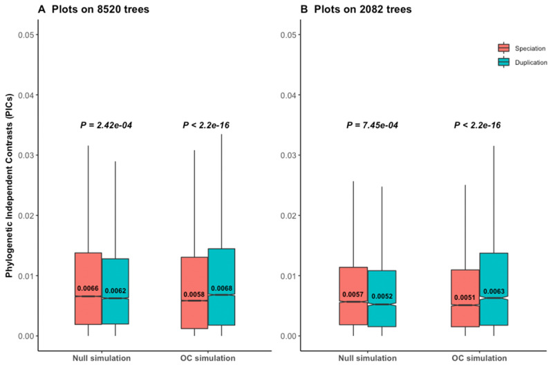
Reanalyses of phylogenetic simulation data of Dunn et al. (2018). P values are from Wilcoxon two-tailed tests. Values inside boxplots denote median PIC values of the corresponding events. In null simulations, there should be no difference in contrasts between events. In OC (ortholog conjecture) simulations, contrasts are expected to be higher for duplication than for speciation. (A) Higher contrasts for speciation than duplication reject the null hypothesis under null simulation scenario for all empirical time calibrated gene trees. (B) Results are similar with a subset of trees with strong phylogenetic signal for $$ \tau $$.

Statistical nonindependence among species trait values because of their phylogenetic relatedness can be measured by phylogenetic signal (Pagel 1999; Freckleton et al. 2002; Blomberg et al. 2003; Münkemüller et al. 2012; Molina-Venegas and Rodríguez 2017). Use of the PIC is mainly important for the data sets with strong phylogenetic signal, where it allows to recover phylogenetically independence. Dunn et al. (2018) used Blomberg’s K. Its value ranges from 0 to $$ \mathrm{\infty }$$ for each tree, where a value of 0 indicates no phylogenetic signal for the trait studied, and a value close to 1 or higher indicates strong phylogenetic signal (Pagel 1999; Freckleton et al. 2002; Blomberg et al. 2003; Münkemüller et al. 2012; Molina-Venegas and Rodríguez 2017). With a cutoff of K > 0.551, Dunn et al. (2018) obtained only 2,082 trees (table 1), 24.4% of the total, with strong phylogenetic signal. The phylogenetic method still rejects the null hypothesis under null simulations for those 2,082 trees using a Wilcoxon two-tailed rank test (fig. 1B), showing that the problem is not simply due to low phylogenetic signal. Using a cutoff of P < 0.05 together with K > 0.551 leads to 1,135 statistically significant trees with strong phylogenetic signals, for which we obtained a similar result (supplementary fig. S3, Supplementary Material online). This means that the bias is not limited to the selection of tree sets, or to the number of speciation or duplication events used for the analyses. As the trend was similar for these 1,135 trees, we continued analyses with the 2,082 trees of Dunn et al. (2018) for consistency.

The accuracy and performance of the PIC method largely depend on proper branch length calibration in absolute time (e.g., in million years—My) (Garland 1992; Díaz-Uriarte and Garland 1998; Cooper, Thomas, FitzJohn, et al. 2016). We thus investigated possible biases created during calibration of gene trees. Due to nonavailability of external references for duplication time points (e.g., no fossils), Dunn et al. (2018) used only seven speciation time points to calibrate substitution rate trees. The ages of other node events are estimated using penalized likelihood (Sanderson 2002) and vary for the same duplication clade labels even within the same gene trees. The oldest speciation age for their calibrated trees was 296 My (table 1), corresponding to the use of chicken as the outgroup. Surprisingly, the calibrated node age of the oldest duplication event was 11,799,977 My (table 1 and supplementary table S1, Supplementary Material online), that is, 2,600 times older than the Earth. This is indicative of issues with time calibration. It is due to the fact that pruning was done prior to the time calibration in Dunn et al. (2018). Pruning to species with τ data leads to trees with many duplication (or NA) nodes older than 296 My. If there were older (>296 My) speciation events before pruning, they are also removed (supplementary fig. S4A, Supplementary Material online). If the root node of a pruned tree is a speciation, the duplication ages are constrained by this speciation. Otherwise, there are no constraints for the duplication events older than the oldest speciation events (supplementary fig. S4 and table S1, Supplementary Material online), which can introduce a calibration bias. This unreliable branch length estimation for the old duplication nodes eventually led to much larger expected variances for gene duplication events than for speciation events (supplementary fig. S5A and B, Supplementary Material online).

PIC of a node is a ratio of changes in trait values ($$ \tau $$ here) for descendant nodes to their expected variance, that is, the lengths of the two branches that connect the node to its two descendants. In this study, lower contrasts refer to lower PIC values, whereas the lower contrasts variance means lower calibrated branch lengths. This means that similar changes in $$ \tau $$ for two nodes can produce different PIC values, with the lower contrast for the node with higher expected variance (i.e., calibrated branch length). In the null simulations only the $$ \tau $$ values are simulated, whereas the branch lengths (hence the expected variances) are taken from the empirical data, and thus share its biases. This explains why contrasts are lower for duplications than for speciations under null simulations as well as with empirical data. Such calibration bias in branch lengths violates the second assumption of PIC applicability and inflates type I error rates (Díaz-Uriarte and Garland 1996, 1998).

Randomization Tests to Assess the Performance of Phylogenetic Method

We used randomization tests to assess bias in different analyses of the empirical data set. Our expectation is that the trend of the empirical result should differ from the randomized ones. In a first randomization test, we permuted the $$ \tau $$ values across the tips of each tree without altering the node events of the trees. By such randomization, the real phylogenetic relationships between trait values are removed for each tree. When we compared the node contrasts of the speciation and duplication events computed based on these 8,420 randomized $$ \tau $$ trees (fig. 2A), we found the same pattern as reported for the empirical gene trees by Dunn et al. (2018), contrary to expectation. It confirms that results are driven by their large differences in branch lengths (i.e., in expected variances) (fig. 2B), as on simulated null data. Any effect of trait divergence rates of speciation and duplication events is always masked by this branch length difference of node events. This violates the basic assumption of applicability of the PIC method to Brownian trait evolution. To remove the problem of difference in expected variances of the two events, we performed a second randomization test: We kept the original $$ \tau $$ value for tips but randomly shuffled the events (duplication, speciation, or NA) of internal nodes of the 8,420 empirical gene trees to maintain the original proportions of speciation and duplication events. The resulting trend (fig. 2C) still resembled the empirical gene trees data. This appears due to the fact that the majority of the nodes are speciations (fig. 2D and table 1) with node ages $$ \le $$296 My. Most of the trees with many duplication events on the other hand have ancient duplication events for which the evolutionary rates of duplication are often masked by the effect of longer branch lengths. Opposite to our expectation, the calibrated trees with no or few duplications have higher overall nodes contrast (apparent fast evolution) than trees with many duplications (apparent slow evolution). This might be due to greater difficulty in detecting paralogs for fast-evolving genes. Therefore, reshuffling of events may not change the observed pattern of higher speciation contrasts than duplication contrasts.

Fig. 2.

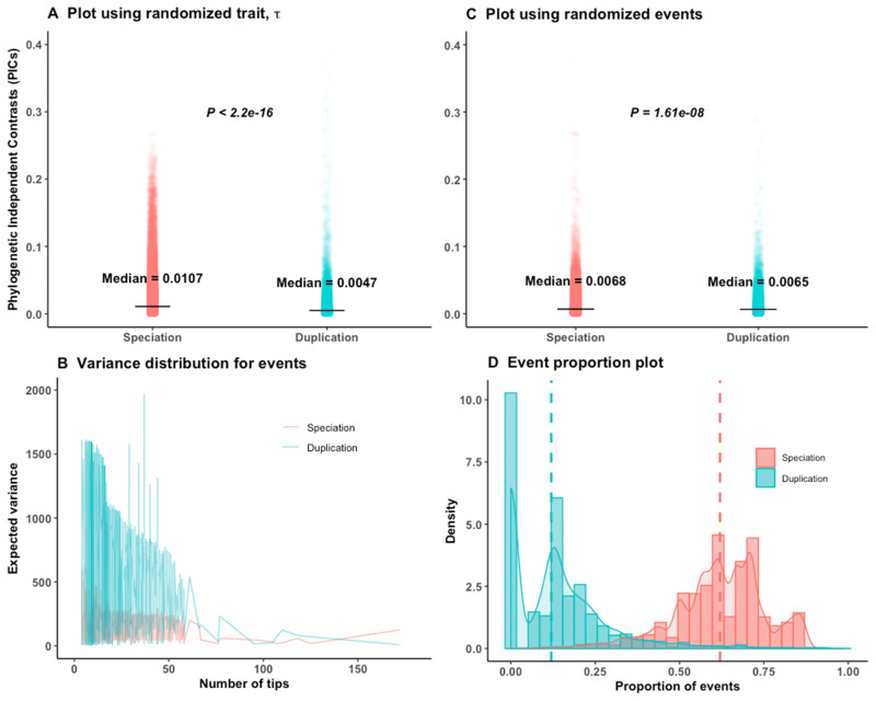
Analyses on calibrated empirical gene trees of Dunn et al. (2018). P values are from Wilcoxon two-tailed tests. (A) Randomly shuffling the $$ \tau $$ values of the tips for 8,520 gene trees does not alter the empirical trend of an opposite trend to the ortholog conjecture. (B) The expected variance is much higher for duplication than speciation events irrespective of the number of tips considered for the study. (C) Using the original $$ \tau $$ data, if we permute the events (Speciation or Duplication or NA) of the nodes, the trend of result remains. (D) The proportion of speciation events is much higher than duplication events for all time-calibrated trees; the dotted line represents the median proportion of both events; a high proportion of trees have no duplication events.

Out of 8,520 calibrated trees, 2,990 were pure speciation trees with no duplication events. For these 2,990 trees, random shuffling of events had no impact. To avoid this bias, we removed those 2,990 speciation trees as well as trees with negative branch lengths and randomized the trait or the internal node events 100 times on the remaining 5,479 trees. However, we still always obtained significantly higher contrasts of speciation than of duplication (supplementary fig. S6A and B, Supplementary Material online). The randomization pattern is the same restricting to 2,082 trees with strong phylogenetic signal (supplementary fig. S6C and D, Supplementary Material online).

All these analyses indicate that the results reported by Dunn et al. (2018) are biased by the calibrated phylogeny structures and that this bias is not easy to correct. We propose three approaches to correct for this bias and recover a proper phylogenetic signal of trait evolution.

Approach 1: PIC with Diagnostic Tests

Diagnostic tests for each tree are essential to ensure phylogenetic independence of node contrasts, especially as there is evidence of bias in the calibrated trees. This can be verified by absence of correlation between the absolute value of PICs and their standard deviations, node height, node age, or node depth (Garland 1992; Garland et al. 1992; Díaz-Uriarte and Garland 1996, 1998; Freckleton 2000; Freckleton and Harvey 2006; Cooper, Thomas, FitzJohn, et al. 2016). A statistically significant negative or positive correlation in any of the diagnostic tests confirms that the PICs for that tree are nonindependent (Garland 1992; Garland et al. 1992; Díaz-Uriarte and Garland 1996, 1998; Freckleton 2000; Freckleton and Harvey 2006; Cooper, Thomas, FitzJohn, et al. 2016); in practice, we used P < 0.05 for significance.

We performed such diagnostic tests on 4,288 trees, for which calibration biases are fixed for old duplication nodes (see Materials and Methods, table 1). Among them only 2,088 (48.7%), which includes 15,321 speciation and 6,213 duplication nodes, passed all four diagnostics tests for $$ \tau $$ evolution. We performed our PIC analyses separately for 3,948 young (≤296 My, the oldest speciation in the trees) and 2,265 old (>296 My) duplication events. Analyses on young duplicates after diagnostic tests provided support for the ortholog conjecture (fig. 3), but old duplicates did not. Randomization tests showed patterns distinct from real data only for the young duplicates (supplementary fig. S7A and B, Supplementary Material online), indicating a biological pattern rather than a data bias. Thus PIC on the trees after diagnostic plot tests supports the ortholog conjecture for young duplicates, whereas the inference remains biased for older duplicates.

Fig. 3.

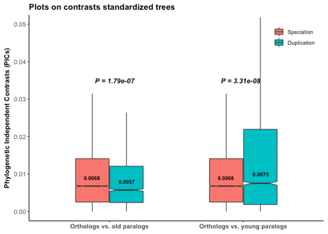
The ortholog conjecture test on $$ \tau $$ for trees passing diagnostic plot tests. P values are from Wilcoxon two-tailed tests. Values inside boxplots denote median PIC values of the corresponding events. Young duplicates: age ≤ 296 My, the maximum speciation age; old duplicates: age >296 My.

Approach 2: PIC with Branch Length Transformation

Most phylogenetic methods are developed for the Brownian model of trait evolution, including PIC (Felsenstein 1985; Cornwell and Nakagawa 2017). Deviations from pure BM violate the fundamental assumptions of PIC applicability and can affect its performance for testing hypotheses about correlated evolution (Garland 1992; Garland et al. 1992; Díaz-Uriarte and Garland 1996, 1998). Using model fitting (see Materials and Methods), we found that 75.6% gene trees (supplementary fig. S8, Supplementary Material online) supported the OU model. Remedial measures, such as branch length transformations and diagnostic tests, can substantially recover the performance of the PIC methods when character evolution is not BM, or when contrasts are nonindependent of the phylogeny (Garland et al. 1992; Díaz-Uriarte and Garland 1996, 1998).

We thus applied branch length transformation on all 4,288 trees, along with diagnostic tests for consistency. The 4,190 trees (97.7%) which pass diagnostic tests after branch length transformation support the ortholog conjecture (fig. 4A). Due to the lack of absolute age for these transformed trees, we did not distinguish young and old duplicates. Applying such branch length transformation then diagnostic tests to the gene trees of Dunn et al., we also found support for the ortholog conjecture in 98.8% (8,417 out of 8,520) (supplementary fig. S9A, Supplementary Material online), as well as for 99.9% (2,080 out of 2,082) of their trees with strong phylogenetic signal (supplementary fig. S10A, Supplementary Material online). Randomization tests on all these sets of trees following branch length transformations clearly showed distinct patterns compared with the empirical data (fig. 4B and C; supplementary figs. S9B, S9C, S10B, and S10C, Supplementary Material online), indicating that results are not due to inference bias once the data are properly transformed.

Fig. 4.

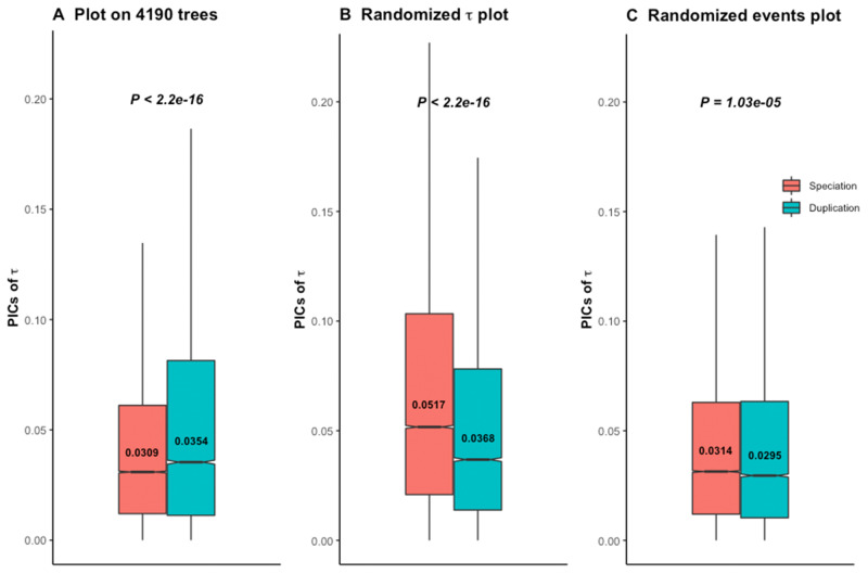
The ortholog conjecture test for contrasts standardized branch transformed trees. P values are from Wilcoxon two-tailed tests. Values inside boxplots denote median PIC value of the corresponding event. (A) Using 4,190 out of 4,288 calibrated trees that passed diagnostic tests following branch length transformation. (B) Permuting τ and (C) permuting internal events on contrasts standardized branch length transformed trees produce distinct patterns compared with the empirical gene trees of (A).

Approach 3: Phylogenetic Data Modeling

State-dependent model fitting allows to compare the evolutionary rates ($$ \sigma $$²) and the changes in adaptive optimum value (θ) associated with specific states (speciation or duplication) for each tree (Beaulieu et al. 2012; Clavel et al. 2015). Under the ortholog conjecture, our expectation is that there should be more shifts in optimum value of $$ \tau $$ between paralogs than between orthologs. Moreover, the evolutionary rates after duplication should be higher than after speciation ($$ \sigma $$²_duplication > $$ \sigma $$²_speciation). Of course, trends on empirical data should differ from randomized ones. When we modeled the evolution of $$ \tau $$ (see Materials and Methods), 32 out of 4,288 trees failed to fit any model due to invariance in $$ \tau $$. Among the others, 308 supported BM1, 704 BMM, 2,874 OU1, and 370 OUM, as the best-fit models (supplementary fig. S8, Supplementary Material online). We performed our analyses separately for young and old duplicates.

On the 8.6% multi optima trees (OUM) the optimum value are significantly higher for duplications, both young and old (θ_dup > θ_spe) (supplementary table S2, Supplementary Material online). Thus, paralogs shift toward higher tissue specificity. These results are not observed on randomized trees, supporting a biological pattern in the data (supplementary table S2, Supplementary Material online).

We also applied a Bayesian method (Uyeda and Harmon 2014) to quantify the number of adaptive optimum shifts, as suggested for small trees (Cooper, Thomas, Venditti, et al. 2016). Unlike the other approach, such detection of evolutionary shifts in a phylogeny does not need a priori knowledge of different states on the tree. Using a strict posterior probability threshold of ≥0.7 with this method, we find that most optimum shifts per branch for $$ \tau $$ follow duplications (median after speciation: 0%, after duplication: 12.5%, paired two-sided Wilcoxon rank-sum test P < 2.2e⁻¹⁶). An OU model can often be incorrectly favored over a BM model in a maximum likelihood framework when applied to trees with <200 tips (Cooper, Thomas, Venditti, et al. 2016). Our gene trees have a median of only 15 tips. We thus applied a conservative Bayesian approach on all of the 3,244 trees for which OU was the preferred model (OU1 + OUM). Even with such a strict posterior probability threshold of ≥0.7, 1,101 trees (33.9%) still supported the OUM model, including 901 trees identified as OU1 by maximum likelihood. We detected the same trend of optimum shifts per branch (median after speciation: 2.3%, after duplication: 10%, paired Wilcoxon rank-sum test P < 2.2e⁻¹⁶). These results are largely consistent for both young and old duplicates (table 2; supplementary table S3, Supplementary Material online). However, the rates of optimum shifts are faster only for young duplicates (table 2; supplementary table S3, Supplementary Material online).

Table 2.

Summary Statistics on 1,101 OUM Trees Passing a Posterior Probability Cutoff of ≥0.7 in a Bayesian Framework.

Duplication Age	Proportions of Regime Shifts per Branch		Paired Two-Sided Wilcoxon Rank Sum Test	Regime Shift Rates (shifts/My)		Two-Sided Wilcoxon Rank Test
	After Speciation	After Duplication		After Speciation	After Duplication
Young	3.1%	4.5%	3.4e−12	0.013	0.031	1.7e−11
Old	2.6%	10%	<2.2e−16	0.013	0.0023	<2.2e−16

Note.—Above analyses include 13,824 speciation, 3,027 young, and 2,814 old duplication events. Values shown in the table indicate median values. The difference in proportions of regime shifts per branch after speciation events for two types of duplications is due to the different sets of trees used. Few trees shared both types of duplicates. Proportion of regime shifts per branch of events is estimated for each tree, and thus paired Wilcoxon test is used to compare the difference. A single gene tree can have multiple-optima shift rates for events, and thus two-sided Wilcoxon rank test was used for comparison.

Analyses on the trees where $$ \sigma $$² varies between events (BMM) also support the ortholog conjecture for young duplicates (table 3). Randomized data showed distinct patterns from empirical data. However, again there was neither support for the ortholog conjecture nor signal relative to randomization for the old duplicates.

Table 3.

Summary Statistics for Brownian Trees.

Duplication Age	Data	σ2Speciation	σ2Duplication	σ2Duplication/σ2Speciation	P-value
Young	Empirical (nSpeciation= 4,642; n Duplication = 1,742)	9e−5	1.4e−4	1.5	5e−12
	Randomized τ (nSpeciation= 4,618; n Duplication = 1,723)	6.9e−4	2.2e−4	0.32	1.4e−13
	Randomized events (nSpeciation= 3,215; n Duplication = 1,438)	1.7e−4	8.5e−5	0.5	0.02
Old	Empirical (nSpeciation= 5,356; n Duplication = 1,295)	1.7e−4	2e−9	1.2e−5	<2.2e−16
	Randomized τ (nSpeciation= 5,337; n Duplication = 1,291)	9.1e−4	2.5e−10	2.7e−7	<2.2e−16
	Randomized events (nSpeciation= 2,788; n Duplication = 800)	1.8e−4	2.1e−9	1.2e−5	<2.2e−16

Note.—Median values of σ² are shown; P-value from paired two-sided Wilcoxon test.

Data Reproducibility Details

Our analyses are based on 21,124 gene trees obtained from ENSEMBL Compara v.75 (Herrero et al. 2016) as used by Dunn et al. (2018). We used the same random seed number as in Dunn et al. (2018) to reproduce the simulation results for reanalysis. All reproduced data of Dunn et al. were stored in the “manuscript_dunn.RData” file (https://doi.org/10.5281/zenodo.4003391). We used the results stored in the “data” or “phylo” slot of the trees for further analyses. To differentiate our own function from theirs (Dunn et al. 2018), we renamed the original function script of Dunn et al. from “functions.R” to “functions_Dunn.R.” We made separate scripts for PIC analyses (Premanuscript_run_TMRR.R) and data modeling analyses (Model_fitting.R). Some of the analyses were time consuming, so we stored our outputs in “Analyses_TMRR.RData” and “Model_fitting_TMRR.Rdata” files (https://doi.org/10.5281/zenodo.4003391) to load during analyses. All the details of different functions are provided inside the scripts. We supply all the previously stored data (to reduce computation time during reproduction of result) and function files including our own (functions_TM_new.R) with this study. All scripts are available on GitHub: https://github.com/tbegum/Testing_the_ortholog_conjecture.

Fixing Time Calibration Bias of Duplication Nodes

We first present the approach that Dunn et al. (2018) used, for clarity. When two speciation nodes had the same label in the gene tree, Dunn et al. edited the more recent one to “NA” rather than “speciation.” Indeed the presence of the same clade names at different node depths forces all the intervening branches to have length zero when the tree is time calibrated, leading to failure of calibration (Dunn et al. 2018). For trait evolution, they annotated the tips of these modified trees with precomputed tissue specificity data,$$ \mathrm{ }\tau $$ from eight vertebrate species (human, gorilla, chimpanzee, macaque, mouse, opossum, platypus, and chicken) (from Kryuchkova-Mostacci and Robinson-Rechavi [2016]). $$ \tau $$ is a univariate index between 0 and 1 that measures tissue specificity of gene expression (Yanai et al. 2005): $$ \tau $$ close to 1 indicates high tissue specificity, whereas close to 0 indicates more ubiquitous expression. Here, $$ \tau $$ was computed across six tissues: brain, cerebellum, heart, kidney, liver, and testis, based on the RNA-seq data of Brawand et al. (2011). Dunn et al. pruned the gene trees to remove tips with missing $$ \tau $$ data and then time calibrated them using speciation clade ages in the chronos() function with the “correlated” model from the R package “ape” (Paradis et al. 2004). The modified NA clades were not used for this calibration. They used seven speciation time points with a maximum age of 296 My. Thus, they obtained 8,520 calibrated gene trees having at least four tips with nonnull trait data (table 1; supplementary fig. S4A–C, Supplementary Material online). Among these trees, 2,990 were pure speciation trees, which include 12,919 speciation events, or 19% of all speciation nodes.

Relative to Dunn et al., we exchanged the order of pruning and time calibration steps, that is, we first time calibrated the 21,124 modified (i.e., with NA added) gene trees, followed by pruning to have at least four tips with $$ \tau $$ data. This makes use of all 32 available speciations time points and helps to limit the calibration bias of the old duplication events (supplementary fig. S4D–F, Supplementary Material online). Calibration fails for some trees, and we obtained 7,336 calibrated gene trees. The maximum node age of old duplication events is 1,175.2 My for these trees, as opposed to 11,799,977 My (older than the universe) for the trees obtained by the original approach (table 1; supplementary table S1, Supplementary Material online). Among these 7,336 gene trees, we kept 4,288 which have at least one speciation and one duplication events; we removed 39 pure duplication and 3,009 pure speciation trees. This 4,288 gene tree set is our basis for evaluating phylogenetic methods’ capacity to test the ortholog conjecture (table 1): We compare the evolutionary rates, $$ \sigma $$², or PICs of speciation and duplication events of the same genes.

Model Selection for $$ \mathit{\tau }$$ Evolution

We followed a state-dependent model-fitting approach to identify BM or OU trees. We classified time-calibrated gene duplication nodes as “young” (≤296 My, the maximum speciation age) or “old” (>296 My) before model fitting. We performed stochastic mapping of our gene trees by assigning discrete states (“speciation,” “young-duplication,” “old-duplication,” and “NA”) to the branches based on the corresponding ancestral node events using the simmap() function of the phytools R package (Revell 2012). For each mapped tree, we fitted four different models of $$ \tau $$ evolution using maximum likelihood: 1) BM1, a single BM rate of evolution (i.e., σ²_speciation = σ²_{young-duplication} = σ²_{old-duplication}); 2) BMM, a BM with multiple rates of evolution for different events (i.e., different σ² are allowed); 3) OU1, a single optimum OU model (i.e., θ_speciation = θ_{young-duplication} = θ_{old-duplication,} σ²_speciation = σ²_{young-duplication} = σ²_{old-duplication,} α _speciation = α_{young-duplication} = α _{old-duplication}), and 4) OUM, a multi optimum OU model with identical strength of selection and rate of drift acting on all selective regimes (i.e., like OU1 but θ_speciation ≠ θ_{young-duplication} ≠ θ_{old-duplication}).

We used both the mvMORPH (Clavel et al. 2015) and OUwie (Beaulieu et al. 2012) R packages to perform model fitting. Sometimes the information contained within a tree is insufficient with respect to the complexity of the fitted models. This can lead to poor model choice by returning a log-likelihood that is suboptimal and may provide incorrect estimation of one or more model parameters for that tree (Beaulieu et al. 2012). Hence, we included the diagnostics (diagnostic=T or diagn=T) during model fitting. The Eigen values of the Hessian matrix of the diagnostics indicate whether convergence of the model has been achieved or whether the parameter estimates are reliable (Beaulieu et al. 2012). For the BM1, BMM, OU1, and OUM models, we first fitted the model using mvMORPH for each gene tree. If any of the models failed to converge for the tree or if the Eigen values of the Hessian matrix indicated that it was not reliable, we refitted that model using OUwie to include it in model comparison. If still it failed, we removed that model for that tree. For model comparisons on each gene tree, we calculated the Akaike weights (ω) for each fitted model by means of the second-order Akaike information criteria (AICc), which includes a correction for small sample sizes (Akaike 1974; Burnham and Anderson 2002). The model with highest ω was selected as the best-supported model of $$ \tau $$ evolution for the tree (Burnham and Anderson 2002; Gearty et al. 2018). We estimated model parameters for each tree based on the best-fit model.

Bayesian Modeling to Detect Phenotypic Optimum Shift

Regime shifts, that is, shifts of optimal $$ \tau $$ values, in OU models were detected by a Bayesian phylogenetic approach of the bayou R package (Uyeda and Harmon 2014). The reversible-jump phylogenetic comparative approach was used to perform MCMC sampling of locations, magnitudes and numbers of shifts in multiple-optima OU models. We ran MCMC chains for 100,000 generations, and the first 30% of samples were dropped as burn-in. We used a strict threshold of posterior probability ≥0.7 to detect an adaptive shift at a given branch of the phylogeny. For each event (“speciation” or “duplication”), we used a ratio of the number of optimum shifts to the number of branches for that event to estimate the proportions of shifts in a phylogeny.

Randomization Test of $$ \mathit{\tau }$$ Values

For each tree, we used $$ \tau $$ data (column name “Tau” in each tree “data” object) across the tips to carry out our randomization test. To randomize, we permuted the actual $$ \tau $$ data without altering internal node events. The pic() function of the “ape” package (Paradis et al. 2004) was used to compute PIC of nodes for each tree using permuted $$ \tau $$ of tips. For each run, we compared the contrasts of speciation and duplication events of the whole set of randomized trees to estimate difference in event contrasts based on Wilcoxon signed rank test. For 100 runs, we repeated the above process 100 times to obtain a distribution plot of 100 independent P values. For our model-fitting approach, we used the same empirical simmap trees with permuted $$ \tau $$ data at the tips. We reestimated the model parameters of the randomized $$ \tau \mathrm{ }$$trees using the best-fit model chosen for the corresponding empirical gene trees.

Randomization Test of Node Events

Some of the speciation nodes had daughters with same clade names in the gene trees we used for our study. Dunn et al. changed such node events to “NA” to avoid problems during time calibration of the trees. Such annotated node event information (“Speciation,” “Duplication,” “NA”) for each tree was available as “Event” in the tree “data” slot. To randomize, we permuted the internal node events (added as column name “event_new” in the “data” slot) by maintaining the actual proportion of events for each tree. Then, we used the PIC of actual $$ \tau $$ at tips to estimate contrasts difference between newly assigned speciation and duplication node events by Wilcoxon rank tests. For 100 independent runs, we repeated the same procedure to obtain 100 independent P values. As the internal node events were changed after such randomization, we reclassified gene duplication nodes as “young” or “old” on the event modified trees and repainted the trees. We reestimated the model parameters for the discrete states of the randomized event trees using the best-fit model chosen for the corresponding empirical gene trees.

Checking for Contrasts Standardization by Diagnostic Tests

We used several additional diagnostic tests on those trees to identify adequate independent nodes contrast standardization before drawing any inference by PIC method, as recommended in several studies (Garland 1992; Díaz-Uriarte and Garland 1996, 1998; Freckleton and Harvey 2006; Cooper, Thomas, FitzJohn, et al. 2016). The most usual method for contrasts standardization is to check a correlation between the absolute values of PICs and their expected standard deviations (i.e., square root of sum of branch lengths) (Garland et al. 1992; Díaz-Uriarte and Garland 1998; Cooper, Thomas, FitzJohn, et al. 2016). Under BM, there should be no correlation. This correlation test and another between the absolute values of PICs and the logarithm of their node age are model diagnostic tests in the caper (Comparative Analyses of Phylogenetics and Evolution in R) package (Purvis and Rambaut 1995; Cooper, Thomas, FitzJohn, et al. 2016; Orme 2018; R Core Team 2018). We used both of them by using the “crunch” algorithm of the caper package, which implements the methods originally provided in CAIC (Purvis and Rambaut 1995; Cooper, Thomas, FitzJohn, et al. 2016; Orme 2018; R Core Team 2018). Correlation of node heights with absolute values of contrasts or PICs has also been reported to be a reliable indicator of deviation from the Brownian model (Freckleton and Harvey 2006). Hence, we computed node height for each node in a tree using the ape package (Paradis et al. 2004). We also used the correlations of node height and node depth to the absolute value of nodes contrasts to rule out significant trend in any of the four tests. We used P < 0.05 to assess a significant correlation for the diagnostic tests. A significant trend (positive or negative) indicates phylogenetic dependence for that tree (Garland 1992; Garland et al. 1992; Díaz-Uriarte and Garland 1998; Freckleton and Harvey 2006; Cooper, Thomas, FitzJohn, et al. 2016), and we removed those trees from our analysis. Contrast calculation on negative branch lengths is not desirable, so we removed trees with negative branch lengths before applying the crunch() function. To assure that nodes contrast standardization is independent of the phylogeny, we considered sets of trees passing all four diagnostic tests for further analyses.

Branch Length Transformation

Transformation of branch lengths has been proposed to restore the performance of PIC method when the true evolutionary model is not BM or is unknown, or when branch lengths are in error (Garland et al. 1992; Díaz-Uriarte and Garland 1996, 1998). In such cases, branch lengths are transformed by raising a family power of branch length ranging from 0 to 2 in intervals of 0.1, plus the log₁₀ of the branch lengths (Díaz-Uriarte and Garland 1996, 1998). For each transformation, the program computes the correlation between the absolute value of the standardized contrasts and their standard deviations until no significant correlation is obtained, to ensure adequate independent contrasts standardization (Díaz-Uriarte and Garland 1996, 1998). Finally, we excluded trees for which adequate contrasts standardization is not achieved even after raising the branch length power to 2 (Díaz-Uriarte and Garland 1996, 1998).

Details of Other Packages Used in This Study

We used phylosig function() of the phytools package (Revell 2012) to identify trees with phylogenetic signal (P < 0.05) using Blomberg’s K (Blomberg et al. 2003; Münkemüller et al. 2012; Revell 2012). Analyses and plotting were performed in R version 3.5.1 (R Core Team 2018) using treeio (Guangchuang 2018), ggtree (Guangchuang et al. 2017), stringr (Wickham 2019), digest (Antoine Lucas et al. 2018), dplyr (Wickham et al. 2017), tidyverse (Wickham 2017), ggrepel (Slowikowski 2018), gtools (Warnes et al. 2018), ggplot2 (Wickham 2016), cowplot (Wilke 2019), easyGgplot2 (Kassambara 2014), gridExtra (Auguie 2017), and png (Urbanek 2013) libraries.