Prediction of the spread of Corona-virus carrying droplets in a bus - A computational based artificial intelligence approach

Mehrdad Mesgarpour, Javad Mohebbi Najm Abad, Rasool Alizadeh, Somchai Wongwises, Mohammad Hossein Doranehgard, Saeidreza Ghaderi, Nader Karimi

https://doi.org/10.1016/j.jhazmat.2021.125358, Volume: 413, Pages: 125358-125358

Article Type: Research Article Article History

Publisher: Published by Elsevier B.V.

- Facebook
- Twitter
- Linkedin
- Whatsapp
Altmetric

Table of Contents

Nomenclature
1 Introduction
2 Problem definition
3 Governing equation
4 Artificial Inteligence
5 Characteristics of sneezing process
6 Results and discussion
7 Conclusions
CRediT authorship contribution statement
Declaration of Competing Interest
Appendix A Supplementary material

Abstract

Public transport has been identified as high risk as the corona-virus carrying droplets generated by the infected passengers could be distributed to other passengers. Therefore, predicting the patterns of droplet spreading in public transport environment is of primary importance. This paper puts forward a novel computational and artificial intelligence (AI) framework for fast prediction of the spread of droplets produced by a sneezing passenger in a bus. The formation of droplets of salvia is numerically modelled using a volume of fluid methodology applied to the mouth and lips of an infected person during the sneezing process. This is followed by a large eddy simulation of the resultant two phase flow in the vicinity of the person while the effects of droplet evaporation and ventilation in the bus are considered. The results are subsequently fed to an AI tool that employs deep learning to predict the distribution of droplets in the entire volume of the bus. This combined framework is two orders of magnitude faster than the pure computational approach. It is shown that the droplets with diameters less than 250 micrometers are most responsible for the transmission of the virus, as they can travel the entire length of the bus.

Keywords

COVID-19, prediction, Droplet distribution, Large eddy simulations, Deep neural network

Mesgarpour,Abad,Alizadeh,Wongwises,Doranehgard,Ghaderi,and Karimi: Prediction of the spread of Corona-virus carrying droplets in a bus - A computational based artificial intelligence approach

Nomenclature

$AI$	Artificial intelligence
$C_{1 M}^{2 σ}$	Vapor mass concentration of the surface
$C_{1 M}$	Mass concentration of a gaseous component
$C_{D}$	Drag coefficient of droplets
$C_{M 1}^{3 σ}$	Partial surface concentration of the vapor
$c_{3}$	Constant parameter
$D$	Hydraulic particle diameter
$D_{3}$	Constant parameter
$D_{M \to \sum n}$	Hydraulic diameter for droplet
$d_{p}$	Diameter of the droplet
$F_{Body}$	Body force
$F_{Drag}$	Drag force
$F_{Added}$	External force
$g$	Gravity
$H^{m^{*}}$	Enthalpy for n^th fluid
$H^{m}$	Enthalpy by the combination of phase-weighted
$h_{M 1}^{3 σ}$	Specific enthalpy for liquid (phase 1)
$h_{M 3}^{3 σ}$	Specific enthalpy for vapor (phase 3)
$h_{fg}$	Enthalpy of vaporization
$h$	Specific enthalpy
$J_{w}$	Evaporation of droplet
$k$	Turbulence kinetic energy
$m^{*}$	m^th fluid phase
$p_{M 1}^{3 σ}$	Partial surface pressure of the vapor
$P_{w}$	Partial saturated vapor pressure
$P_{V, i, U}$	Ratio of the volume of all the particles with diameters in size class I
$p$	Pressure
$P_{a}$	Partial water vapor pressure
$q_{H}^{m^{*}}$	Heat flux for n^th fluid (droplet enthalpy)
$q^{m^{*}}$	Heat flux for n^th fluid
$RH$	Relative humidity
$Re$	Reynolds number
$S_{m^{m^{*}}}^{int},$	The interface between phases for mass
$S_{u^{m^{}}}^{m^{}}, S_{v^{m^{}}}^{m^{}}, S_{w^{m^{}}}^{m^{}}$	Source or sink terms
$S$	Rate of strain tensor for the resolved scale
$T_{ambient}$	Temperature
${∆ T}^{m}$	Mixture temperature gradient
$T_{3}^{1 σ}$	Vapor temperature (partial surface)
$u^{m^{}}, v^{m^{}}, w^{m^{*}}$	Velocity component for n^th fluid
$V$	Airflow velocity
$t$	Time
$U^{dr, m^{*}}$	Drift velocity vector of the k^th phase
$U_{wall}$	Wall velocity
$u_{t}$	Tangential velocity component
$U^{m}$	Mixture velocity
$V_{ins}^{f}$	Volume of fluid (initial state)
$V_{ins}^{p}$	Volume of the second phase (initial state)
$V_{a}$	Air velocity
$V_{p}$	Volume of the second phase
$x - y - z$	Coordinates, m

Greek symbol

$Θ$	Stress field for the two phase flow
$β$	Slip coefficient
$α^{m}$	Volume fraction of the mixture
$α^{m^{*}}$	Volume fraction for N^th fluid phase
$μ_{T}^{m^{*}}$	Turbulent viscosity of the continuous n^th phase
$ρ^{m^{*}}$	Density for n^th fluid
$μ^{m^{*}}$	Viscosity for n^th fluid
$α_{3}$	Constant parameter
$ε$	Turbulence dissipation
$μ_{m}$	Mixture viscosity
$ζ$	Relaxation factor (functional)
$Γ^{m^{*}}$	Favre-averaged quantity
$λ^{m^{*}}$	Thermal conductivity for n^th fluid phase
$σ$	Capillary force
$τ$	Response time
$ρ^{f}$	Fluid density
$ρ^{m}$	Mixture density
$λ^{m}$	Mixture thermal conductivity
$ρ$	Density
$ρ_{l}$	Density of the liquid phase

1 Introduction

The spread of Corona-virus via droplets generated by human sneezing and coughing has attracted a significant attention in recent months. It has been shown that this process can enhance the virus transmission by 18 times (Chen, 2020, Meccariello and Gallo, 2020, Diwan et al., 2020, Rockett et al., 2020). Dispersion of the droplets produced by human sneezing is a complex physical process (Enserink and Kupferschmidt, 2020, Ivorra et al., 2020). Upon leaving the mouth, the saliva droplet is broken down into smaller droplets. The subsequent evaporation of droplets and reduction of diameters cause drastic changes in their deposition and suspension. This highly complicates the development of predictive models for spread of such droplets and the subsequent transmission of the virus (Chaudhuri et al., 2020, Abuhegazy et al., 2020).

A considerable amount of work has been already done on modelling of sneezing. In 2019, Hassani and Khorramymehr (2019) studied the process of transmitting sneezing generated droplets into human airways. The results showed that for an average flow rate of 4.79 L/s, the airflow outlet velocity from the mouth reaches 5.3 and 8.4 m/s, respectively. In 2020, Singh and Tripathi (2020) numerically simulated the dispersion of sneezing particles in a room. Their investigation was complimented by an experiment and put forward a model for measuring the transfer of particles in surrounding air. This was continued by Kotb and Khalil (2020) with a numerical study of the emission of particles containing SARS-COVID 19 virus into the interior of a passenger aircraft. The result indicated that velocity of the droplets produced by the moving passengers could reach the seated passengers. However, sneezing generated droplets had more harmful impacts than those produced by coughing, while both traveled a long distance inside the cabin.

Most recently, Busco et al. (2020) conducted a comprehensive study of the spread of the virus in the environment and showed that the deposition of different particles is a function of their average diameter. They further argued that environmental effects play a major role in particle dispersion. In another study, Li et al. (2020) investigated the emission model of sneezing droplets and concentration of the resultant particles in the environment. Through an analysis of the effects of ventilation on the spread of the virus in a room, Ali Hasan (Hasan, 2020) showed that the intensity and direction of airflow inside the room significantly affect the dispersion model. Chaudhuri et al. (2020) developed a model of droplet distribution based on reaction. Their model was validated against the experimentally obtained evaporation data of levitated droplets of pure water and salt solution. As expected, the droplet evaporation time was found to be dependent on the ambient temperature and was also a strong function of relative humidity. Verma et al. (2020) showed that the use of protective shields can have a significant effect on the pattern of droplets diffusion as well as the spread of contamination in the sneezing process. Abuhegazy et al. (2020) examined the emission model of aerosols in air, and found that these particles could be easily transported in the environment by the ambient flow.

In general, numerical methods provide a convenient framework to study dispersion of the virus carrying droplets. Hence, a number of researchers tried to detect virus transmission routes via numerical simulations (Chen, 2020, Meccariello and Gallo, 2020, Diwan et al., 2020, Rockett et al., 2020, Enserink and Kupferschmidt, 2020, Ivorra et al., 2020, Chaudhuri et al., 2020, Abuhegazy et al., 2020). Table 1 presents an outline of the latest research articles on the applications of computational particle science combined with computational fluid dynamics.

Table 1

List of the most recent investigations that employed a combination of CFD and particle science.

Model	Dimensions	Particle/Droplet size (mm)	Domain	Turbulence method	Target	Solver	Ref.
Unsteady-DPM	2D	0.1–0.3	tube banks	k-ω (SST)	Deposition particle	Ansys Fluent	(Mu et al., 2020)
Unsteady-DPM	2D	0.012	cryogenic condenser	k-ω (SST)	Deposition particle	Ansys Fluent	(Hendry et al., 2019)
Unsteady-Lagrangian particle tracking	2D	0.001–0.01	airway	RANS	Particle flows	Ansys Fluent	(Kim et al., 2019)
Unsteady-DPM	2D	0.001–0.05	ribbed duct air flows	RANS	Particle deposition	Ansys Fluent	(Lu and Lu, 2016)
Unsteady-DPM	3D	0.001–11.25	90-degree bend of natural gas pipelines	k-ω (SST)	Particle deposition	Ansys Fluent	(Seyfi et al., 2020)
Lagrangian Particle Track	2D	0.002–0.058	cyclone separator	RANS	Particle deposition	Ansys Fluent	(Song et al., 2017)
Unsteady-DPM	3D	0.002–0.005	Nose-to-Lung	k-ω (SST)	Aerosol Delivery	Ansys Fluent	(Dutta et al., 2020)
Unsteady	3D	–	environment	LES	Breathing Simulations	Ansys Fluent	(Ivanov and Mijorski, 2019)
Unsteady-DPM	2D	0.001–0.009	lung	LES	Aerosol deposition	Ansys Fluent	(Huang et al., 2020)
Unsteady-DEM	3D	0–0.002	inhalation indoors	Monte-Carlo	SARS-CoV-2 transmission		(Vuorinen et al., 2020)
Lagrangian method	2D	–	combustion	RANS	Ash deposition	In-house code	(Yang et al., 2017)

Public transport contributes significantly to transmission of COVID-19 (Abuhegazy et al., 2020). As a result, there is a substantial emphasis on the mitigation of transmission risk in public transport including buses and train carriages. This, in turn, calls for prediction of the spread of the virus in indoor environments. In general, such predictions can be made by the conventional computational analyses. However, the associated computational burden forbids their use in practical risk assessments. As a remedy, the techniques from machine learning can be utilized to reduce the computational load. This will lead to the development of a data-driven model that uses the computationally generated data for a small section of the domain and extrapolates those. The effectiveness of such combined approach has been already demonstrated in the context of propulsion and process engineering (Christodoulou et al., 2020, Alizadeh et al., 2020a, Mohebbi Najm Abad et al., 2020, Alizadeh et al., 2020b). It was shown that data-driven approaches could predict complicated spatiotemporal behaviors, while high fidelity computation was performed only for a small fraction of the domain (Christodoulou et al., 2020). Hence, the current study includes a computational part followed by artificial intelligence (AI). In the numerical study, computational fluid dynamics is used to model a three-phase flow of liquid droplets and water vapor in air during the droplet distribution process. This model is based on the changes in the particle diameters encountered in sneezing process and their transmission by air flow. Due to the large gradient in the sneezing process and the changes in the flow Reynolds number, an innovative model is developed for low cost and yet accurate analysis of high and low-speed flows. The numerical results are then fed into an AI-based soft tool, which predicts the droplet distribution inside a bus. This results in a novel combination of computational fluid dynamics and artificial intelligence, which forms an efficient tool for practical risk assessments.

2 Problem definition

Buses are the most common means of public transport throughout the world and have specific features that make them pertinent to transmission of the virus. These include the high surface density of passengers and the lack of strong ventilation. In this study, one of the common types of urban buses is considered. Fig. 1 shows a schematic view of the investigated (90 m³ net capacity) bus along with its interior layout. By considering the seats and other components, the internal volume of the bus is about 80 m³. Here, it is assumed that the exit doors are closed. It should be noted that motion of the buses in urban areas is usually slow and does not involve significant accelerations. Thus, any effect made by the motion of the bus has been ignored.

Fig. 1

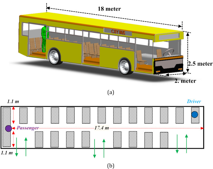
The schematic view of a) the investigated bus and sneezing person, b) seat position and key dimensions.

Fig. 1b shows the locations of the seats. In this configuration, 35 seats with the height of 1.20-meter were considered. Each seat has a 0.5-meter distance from the next one in front and a 10 cm gap on the side. To simplify the simulations, only one infected passenger was considered. As shown in Fig. 1a, a standing passenger (1.80 m of height) at the end of the bus is sneezing. The passenger is located on the center-plane of the bus. Steady-state airflow (V = 0.1 m/s) is injected at the end of the bus. This system is closed and stays at constant temperature and humidity (T_ambient = 20 $℃$ , RH = 20%). All the walls and doors of the bus are assumed to be adiabatic. In the proceeding analysis, all fluids are assumed to be isotropic and Newtonian and, the flow is incompressible.

3 Governing equation

The multiphase flow in this study contains liquid, gas and vapor phases. To model this complex, three phase flow, the conservation of mass and momentum in the Eulerian framework for any $m^{*}$ fluid is written as (Yeoh and Tu, 2019, Kolev and Kolev, 2007, Crowe et al., 2011):

Conservation of mass:

\frac{\partial (α^{m^{*}} ρ^{m^{*}})}{\partial t} + \frac{\partial (α^{m^{*}} ρ^{m^{*}} u^{m^{*}})}{\partial x} + \frac{\partial (α^{m^{*}} ρ^{m^{*}} v^{m^{*}})}{\partial y} + \frac{\partial (α^{m^{*}} ρ^{m^{*}} w^{m^{*}})}{\partial z} = S_{m^{m^{*}}}^{int}

(1)

In this equation, t, is time and x,y,z are the three spatial coordinates.

Transport of momentum in x,y,z directions:

\begin{matrix} \frac{\partial (α^{m *} ρ^{m *} u^{m *})}{\partial t} + \frac{\partial (α^{m *} ρ^{m *} u^{m *} u^{m *})}{\partial x} + \frac{\partial (α^{m *} ρ^{m *} v^{m *} u^{m *})}{\partial y} + \frac{\partial (α^{m *} ρ^{m *} w^{m *} u^{m *})}{\partial z} \\ = \frac{\partial}{\partial x} [α^{m *} (μ^{m *} + μ_{T}^{m *}) \frac{\partial u^{m *}}{\partial x}] + \frac{\partial}{\partial y} [α^{m *} (μ^{m *} + μ_{T}^{m *}) \frac{\partial u^{m *}}{\partial y}] + \frac{\partial}{\partial z} [α^{m *} (μ^{m *} + μ_{T}^{m *}) \frac{\partial u^{m *}}{\partial z}] + S_{u^{m *}}^{m *} \end{matrix}

(2)

\begin{matrix} \frac{\partial (α^{m *} ρ^{m *} v^{m *})}{\partial t} + \frac{\partial (α^{m *} ρ^{m *} u^{m *} v^{m *})}{\partial x} + \frac{\partial (α^{m *} ρ^{m *} v^{m *} v^{m *})}{\partial y} + \frac{\partial (α^{m *} ρ^{m *} w^{m *} v^{m *})}{\partial z} \\ = \frac{\partial}{\partial x} [α^{m *} (μ^{m *} + μ_{T}^{m *}) \frac{{\partial v}^{m *}}{\partial x}] + \frac{\partial}{\partial y} [α^{m *} (μ^{m *} + μ_{T}^{m *}) \frac{{\partial v}^{m *}}{\partial y}] + \frac{\partial}{\partial z} [α^{m *} (μ^{m *} + μ_{T}^{m *}) \frac{{\partial v}^{m *}}{\partial z}] + S_{v^{m *}}^{m *} \end{matrix}

(3)

\begin{matrix} \frac{\partial (α^{m *} ρ^{m *} w^{m *})}{\partial t} + \frac{\partial (α^{m *} ρ^{m *} u^{m *} w^{m *})}{\partial x} + \frac{\partial (α^{m *} ρ^{m *} v^{m *} w^{m *})}{\partial y} + \frac{\partial (α^{m *} ρ^{m *} w^{m *} w^{m *})}{\partial z} \\ = \frac{\partial}{\partial x} [α^{m *} (μ^{m *} + μ_{T}^{m *}) \frac{\partial w^{m *}}{\partial x}] + \frac{\partial}{\partial y} [α^{m *} (μ^{m *} + μ_{T}^{m *}) \frac{\partial w^{m *}}{\partial y}] + \frac{\partial}{\partial z} [α^{m *} (μ^{m *} + μ_{T}^{m *}) \frac{\partial w^{m *}}{\partial z}] + S_{w^{m *}}^{m *} \end{matrix}

(4)

In (1), (2), (3), (4), $α^{m^{*}}, ρ^{m^{*}} and$ $u^{m^{*}}, v^{m^{*}}, w^{m^{*}}$ are the volume fraction, density and flow velocity components of the N^th fluid phase, respectively. Further, $μ_{T}^{m^{*}}$ denotes turbulent viscosity of the continuous N^th phase and $S_{u^{m^{*}}}^{m^{*}}, S_{v^{m^{*}}}^{m^{*}}, S_{w^{m^{*}}}^{m^{*}}$ , are the source terms. The energy equations for the multiphase model (mixture) are:

\begin{matrix} \frac{\partial (ρ^{m} H^{m})}{\partial t} + \nabla . (ρ^{m} U^{m} w^{m}) = \nabla . (λ^{m} Δ T^{m}) - \nabla . q_{H}^{m ″} + ζ - \nabla . \sum_{m^{*} = 1}^{2} (α^{m^{*}} ρ^{m^{*}} U^{d r, m^{*}} H^{m^{*}}) \\ ρ^{m} = \sum_{m^{*} = 1}^{2} (α^{m^{*}} ρ^{m^{*}}), λ^{m} = \sum_{m^{*} = 1}^{2} (α^{m^{*}} λ^{m^{*}}) \end{matrix}

(5)

Here, $H^{m}, ζ, U^{dr, m^{*}}$ are enthalpy by the combination of phase-weighted, relaxation factor (functional) and drift velocity vector of the N^th phase, respectively, and the latter is define as $U^{d r, m^{*}} = U^{m^{*}} - U^{m}$ .

The combination of mixture velocity and enthalpy for the phase and mass-weighted variables leads to:

U^{m} = \frac{\sum_{m^{*} = 1}^{2} (α^{m^{*}} ρ^{m^{*}} U^{m^{*}})}{\sum_{m^{*} = 1}^{2} (α^{m^{*}} ρ^{m^{*}})}, H^{m} = \frac{\sum_{m^{*} = 1}^{2} (α^{m^{*}} ρ^{m^{*}} H^{m^{*}})}{\sum_{m^{*} = 1}^{2} (α^{m^{*}} ρ^{m^{*}})}

(6)

3.1 Inter-phase mass transfer

In the vaporization process, if the kinetic energy of droplets and the work of viscosity term are neglected, the transfer of mass on the interface of the droplets and vapor can be reduced to (Ivorra et al., 2020):

{Γ'}^{m^{*}} = \frac{\sum_{m^{*}} \bar{〈 q^{m^{*}} . \nabla_{χ} 〉}}{h_{f g}}

(7)

In Eq. (7), $h_{fg}$ is the enthalpy of vaporization and $q^{m^{*}}$ is the heat flux for N^th fluid. This equation can be defined as the net heat transport to the interface of droplet divided by the latent heat of vaporization process.

3.2 Large eddy simulation (LES)

In LES, the large energy-containing eddies are computed directly (within the accuracy of the computational scheme) and the small-scale structures are modeled. For the bulk multiphase flow, the mathematical formulations consist of a continuous and discrete phase. The Favre-averaged transport equations of mass and momentum utilized in LES are given by (Vuorinen et al., 2020):

(\frac{\partial ρ}{\partial t}) + (\frac{\partial (\bar{ρ u_{i}})}{\partial x_{j}}) = 0

(8)

(\frac{\partial (\bar{ρ u_{j}})}{\partial t}) + (\frac{\partial (\bar{ρ u_{i} u_{j}})}{\partial x_{j}}) = - (\frac{\partial p}{\partial x_{i}}) + (\frac{\partial σ_{i j}}{\partial x_{j}}) - (\frac{\partial τ_{i j}}{\partial x_{j}}) + S

(9)

In Eq. (9), S denotes the body forces acting on the fluid. The subgrid-scale (SGS) stress tensor ( $τ_{i j}$ ) is modeled through an eddy-viscosity approach

\begin{matrix} τ_{i j} \approx ρ (\bar{u_{i} u_{j}} - \bar{u_{i}} \bar{u_{j}}) \\ S_{i j} = \frac{1}{2} (\frac{\partial (\bar{u_{j}})}{\partial x_{i}} + \frac{\partial (\bar{u_{i}})}{\partial x_{j}}) \end{matrix}

(10)

$S_{i j}$ is the rate of strain tensor for the resolved scale. Here, the so called ‘one equation eddy-viscosity model’ (OEEVM) subgrid-scale (SGS) was employed. To calculate the turbulent kinetic energy (K), the OEEVM was solved as follows.

\partial (\bar{ρ} k) + \nabla . (\bar{ρ} k u) = - τ_{i j} . S_{i j} + \nabla . (μ_{k} \nabla k) + \bar{ρ} ε

(11)

ε = c_{3} k^{3 / 2} / Δ

(12)

The kinetic energy in LES turbulence method is defined as:

\begin{matrix} {〈 u_{i} \frac{\partial f_{p}}{\partial f_{p}} 〉}^{*} = u_{i} \frac{\partial {〈 f_{p} 〉}^{*}}{\partial f_{p}} \\ \frac{\partial {〈 f_{p} 〉}^{*}}{\partial t} + u_{i} \frac{\partial {〈 f_{p} 〉}^{*}}{\partial x_{i}} + \frac{\partial}{\partial u_{i}} [\frac{1}{τ_{p}} ({〈 U_{f i} 〉}^{*} - u_{i}) {〈 f_{p} 〉}^{*}] = - \frac{1}{τ_{p}} \frac{\partial {〈 {u^{*}}_{f i} f_{p} 〉}^{*}}{\partial u_{i}} \end{matrix}

(13)

where

{u^{*}}_{f} = (U_{f} | C) - {〈 U_{f} 〉}^{*}

. Using Boussinesq approximation, a simple correlation for the incompressible Reynolds stress tensor is developed, which is expressed by

\bar{\bar{{u'}_{i} {u'}_{j}}} = 2 / 3 k δ_{i j} - v_{T} (\frac{\bar{\bar{{u'}_{i}}}}{\partial x_{j}} + \frac{\bar{\bar{{u'}_{j}}}}{\partial x_{i}})

(14)

3.3 Droplet evaporation process

The evaporation of droplets is modeled using (Chen, 2020, Meccariello and Gallo, 2020, Diwan et al., 2020, Rockett et al., 2020, Enserink and Kupferschmidt, 2020, Ivorra et al., 2020, Chaudhuri et al., 2020, Abuhegazy et al., 2020):

\begin{matrix} J_{w} = 1 \times 10^{- 6} (20.56 + 27.21 V_{a} + 6.392 V_{a}^{2}) {(1 \times 10^{- 3} (P_{w} - P_{a}))}^{b} \\ b = 1.22 - 0.19 V_{a} + 0.0387 V_{a}^{2} \end{matrix}

(15)

In this regard, surface evaporation depends on $V_{a}$ ،, $P_{w}$ and $P_{a}$ , which depend on the air velocity, partial saturated vapor pressure, and partial water vapor pressure in air, respectively.

3.4 Droplet merging

The most common way to achieve the integration of droplets is to ensure that there is an electric field where the two droplets meet. Link et al. (2006) showed that there are direct relations between voltage and rate of merging. This results in oppositely charged surfaces, which will merge the particles together. Also, Chabert et al. studied the merging of individual droplets and particle pairs via electro coalescence (EC)(Chabert et al., 2005). For Newtonian and incompressible fluids at low Reynolds and Bond numbers, this process is defined as (Niu et al., 2008):

μ \nabla^{2} U - \nabla P = \nabla Θ

(16)

with µ being the viscosity of fluid, U the velocity in X direction, P the total pressure and

Θ

the stress field in each phase of the two-phase fluid.

3.5 Boundary conditions

3.5.1 Sneezing profile

As shown in Fig. 2, sneezing involves a sudden change in pressure. The details of this pressure variation depends upon the person’s gender, age and other physiological features. A fluid flow under the pressure trace shown in Fig. 2 is ejected from the mouth. The inner surface of the mouth is a wall and the throat is modelled as a pressure inlet boundary condition. The fluid flow has a relative humidity of 75% and temperature of 35 $℃$ . Unlike previous investigations, here the process of salvia droplet formation through passage of air over the wet surfaces of mouth and lips is fully modeled. According to the geometry of the mouth, the applied pressure leads to an increase in the fluid velocity up to 85 m/s at the lips. The exit location of the mouth was a pressure outlet and a homogenous droplet of saliva distribution, while the physical properties are extracted from Refs. Ericsson and Stjernström, 1951, Briedis et al., 1980. It is further clarified that the no-slip boundary condition was applied to the fluid flow in the mouth.

Fig. 2

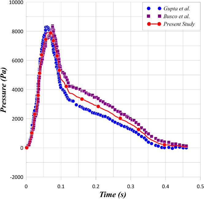
Two models of sneezing pressure profile based on (Gupta et al., 2009) and (Busco et al., 2020) for 20–50 years old person and the average of this model as pressure profile (T_inf=25°C, 25 m/s < Velocity<150 m/s).

3.5.2 Droplet

For each droplet, the shape is affected by the balance of internal and external forces. According to Han et al. (2013) the maximum rate of the volume-based size distributions can be represented by Yeoh and Tu (2019):

P_{V, i, U} = A_{U} (\frac{1}{\sqrt{2 π σ_{U}}}) e^{- (\log_{10} (D_{i}) - μ_{U}) / 2 σ_{u}^{2}}

(17)

In Eq. (17), $P_{V, i, U}$ is the ratio of particle diameters in size class I and $σ$ is the Capillary force. In this simulation, each droplet has two specific features a) variable surface and b) possibility of evaporation and merging.

3.6 Evaporation and droplet merging

For vaporization and condensation processes, if the kinetic energy and viscous work terms are neglected, the interfacial mass transfer can be derived by setting $ζ = 0$ . According to equation (15), the mass flux due to vaporization or condensation can be approximated with the knowledge of heat flux on the interface (Yeoh and Tu, 2019). If the fluid side heat flux to the interface exceeds the vapor side heat flux, vaporization occurs. The reverse applies to condensation. It can be shown that the fluid side interfacial heat flux tends to dominate the process. Using Stefan’s correlation and solving the surface vapor mass concentration for the interface of droplet, the concentration of mass for each phase is (Chen, 2020, Meccariello and Gallo, 2020, Diwan et al., 2020, Rockett et al., 2020, Enserink and Kupferschmidt, 2020, Ivorra et al., 2020, Chaudhuri et al., 2020, Abuhegazy et al., 2020).

C_{1 M}^{2 σ} = 1 - (1 - C_{1 M}) \exp (\frac{D_{3}^{2}}{6 α_{3} ρ_{1} s h D_{M \to \sum n}} \frac{χ_{3}^{1 σ} (T_{3}^{1 σ} - T_{3})}{h_{M 1}^{3 σ} - h_{M 3}^{3 σ}})

(18)

In Eq. (18), $C_{1 M}$ mass concentration of gas component, $h_{M 1}^{3 σ}$ is specific enthalpy for liquid (phase 1) and $h_{M 3}^{3 σ}$ is specific enthalpy for vapor (phase 3).

To calculation the partial surface pressure of the vapor, the concentration equation can be put into the body force equations:

p_{M 1}^{3 σ} = p \frac{C_{M 1}^{3 σ}}{M_{M 1}} / [\frac{C_{M 1}^{3 σ}}{M_{M 1}} + \frac{1 - C_{M 1}^{3 σ}}{M_{1 n}}]

(19)

\begin{matrix} F_{D r a g} = \frac{π}{8} ρ^{f} d_{p}^{2} C_{D} (V_{i n s}^{f} - V_{i n s}^{p}) | V_{i n s}^{f} - V_{i n s}^{p} | \\ F_{A d d e d} = K_{A} ρ^{f} V_{p} \frac{d (V_{i n s}^{f} - V_{i n s}^{p})}{d t} \\ F_{B o d y} = ρ^{p} V_{p} g \end{matrix}

(20)

where

ρ^{f}

, dp Vp,

p_{M 1}^{3 σ}, C_{1 M}^{2 σ}

are the fluid density, particulate diameter, volume of the second phase for a spherical particulate, partial surface pressure of the vapor and surface vapor mass concentration, respectively. Further,

V_{ins}^{p}

is volume of the second phase (the initial state) and

V_{ins}^{f}

denotes the volume of fluid (the initial state).

Due to the complexity of sneezing process, here, a multi-layer flow solver was used. The domain was divided into four parts. In the first part, the internal airflow in the throat and mouth was modeled by employing a single phase RANS, K-epsilon model considering the movement within the oral environment. In this part, a polyhedral mesh structure and the coupling of the SIMPLE velocity and pressure equations were used. Since the configuration involves a single-phase mode at the inlet along with saliva over the entire inner surface of the mouth, a volume-of fluid (VOF) methodology was employed to model the multiphase flow in that region. This renders a hybrid model, which starts as a single-phase flow and gradually turns into a two-phase flow.

In the second part, starting from the mouth and extending for 1 m, LES was utilized to model the spray and dispersion of droplets of saliva. Due to the relatively high velocity of the flow in this section and the presence of vortices, a full structure grid generation has been developed. Included in the model is evaporation and heat transfer within the droplet and the possibility of droplets merging. It is essential to note that unlike most existing studies on modeling of sneezing, here no model of spray or ejector was used. Instead, the entire process of two-phase flow formation was replicated. Liquid droplets were precisely modeled in the space of one meter from the face of the sneezing person. The droplets leaving the mouth cover a wide range of diameter from one to one thousand microns. The statistical distribution of these particles at the moment of exiting the mouth is quite uniform. In the LES region, the second-order precision and QUICK solution model were applied. Also in this area, due to the geometric deformation of the droplets and their movement, an adaptive grid generation was used for each particle movement. The time step was adaptive by location and a time step of 0.0001 s was considered as the basis.

3.7 Concentration and particle diameter measurement (PDM)

Fig. 3 illustrates the method applied to calculate the average value of the droplets in each time step. Based on this, one computational domain for each droplet around the virtual center of mass was considered. This computational domain was fitted to the surface of droplet. The fitting process was based on the adaptive grid generation. A number of vertical vectors on the surface were drawn at any point with the same distribution on the surface, the number of which increased or decreased depending on the particle diameter. The average value of droplet diameter was obtained at any given time in all ranges. The values calculated at each time step were then averaged from all three axes. The amount of virus transmitted by each droplet is directly related to the particle diameter. Therefore, the study of changes and classification of droplets based on their average diameter is an important part of calculating the distribution of droplets in the range of 1–1000 µm. This specific model examines the diameter changes at each time step, which vary by the external and internal forces and evaporation, and provides an ability to statistically evaluate the diameter of the droplets. The developed scheme further offers the ability to calculate the number of particles in a constant volume through applying an image processing technique.

Fig. 3

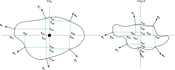
Calculation method for the surface and volume of the droplet by NODE algorithm.

3.8 Validation

Extensive tests confirmed the grid independency of the simulations. Further, a comparison between the current numerical results and those from several well-established computational models and empirical correlations have been presented in Fig. 4. An excellent agreement is evident confirming validity of the numerical simulations.

Fig. 4

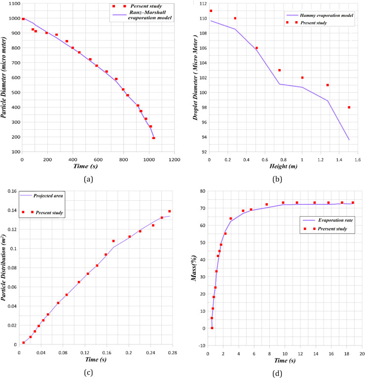
Validation for numerical method base on a) Ranz- marshal equation (Ranz and Marshall, 1952), b) Hamey evaporation model (Hamey, 1982), c) Busco particle distribution (Busco et al., 2020), d) mass profile (Busco et al., 2020).

4 Artificial Inteligence

To predict of the concentration and velocity, a Multi-Input Multi-Output (MIMO) model is developed. In each experiment, several inputs including time, concentration and velocity are given to the model to calculate concentration outputs. The number of input samples in each experiment is about 1240. For prediction, a Deep Neural Network (DNN) regression with a number of input, hidden and output layers was constructed (Schmidt-Hieber, 2020). One superiority of this model is achieving high accuracy on complex data. One of its main challenges is the existence of a weak structural theory (Du and Xu, 2017). In other words, there is no certain theory for the arrangement of elements in a network. Often, the model is studied experimentally and by applying some techniques such as changing the number of layers and neurons and testing different activation functions the accuracy of the model is improved. The sequential models used in this paper have been developed by importing sequential functions from the Keras library of Python. By using the Dense function of the Keras library, 5 layers have been inserted to the network. The first layer is used as the input layer to receive attributes values. Model attributes are: time, location, pressure, temperature and density. In the proposed model, three hidden layers are used, which include 30, 20 and 15 neurons, respectively. The number of neurons and the type of activation functions were selected by several experiments.

Of course, in selecting the appropriate structure for the network, it is useful to use the proposed structures in models that have already been used for DNN regression. The ReLU activation function is used for the neurons of hidden layer, which is one of the most widely utilized and simplest nonlinear activation functions. The two advantages of this function are that it is not saturated with a large number of inputs and the errors are simply back propagate (Schmidt-Hieber, 2020). The last layer of the network is the output layer, which contains some neurons. These neurons return the result of the prediction of concentration and velocity. The defect of the ReLU activation function is that it only takes values for values greater than zero. Thus, the Sigmoid activation function is used in the output layer. Other settings made on the model are the selection of epoch value and batch size. An epoch is a count of the number of times all training data are used once to update neural weights. For batch training, all training samples go through the training algorithm simultaneously at an epoch before the weights are updated. The model weights is updated at the end of each epoch and the batch size. Adam optimizer is also used to calculate the adaptive learning rate for each parameter. This optimizer has been utilized to update the neuron weights of hidden layer.

Finally, the steps of creating the proposed model are presented. At first, the provided dataset is loaded. Then, the data preprocessing is done, which includes data normalization. Then, the sequential model is created. Input, hidden, and output layers are created using the ReLU and Sigmoid activation functions. Afterwards, model compilation is done using Adam optimizer. The epoch value and batch size are determined for the model. Subsequently, the concentration and velocity prediction is done with the model. Finally, the model is evaluated. Tensor flow has been used as a backend to create a predictive model based on deep neural network. It is a library written for high-performance numerical calculations in Python. The Sequential Model API has also been developed and evaluated with Keras and Python3 libraries. Keras is a Python library developed for deep learning. The Sequential model API is utilized to create a model for predicting the concentration and velocity and to which the model layers are added. Also, the Keras Regressor was used to evaluate the model. Performance evaluation was performed using tenfold cross-validation. In this method, the samples are divided into 10 categories. In each step, 9 categories are used to train the model and 1 category is used to test the model. The epoch and batch size values are set to 200 and 5, respectively.

The accuracy of the model is calculated with the criteria of Mean Square Error (MSE) and Mean Absolute Error (MAE). These criteria are calculated as follow:

MAE = \frac{\sum_{i = 1}^{n} |y_{i} - t_{i}|}{n}

(24)

MSE = \frac{\sum_{i = 1}^{n} {(y_{i} - t_{i})}^{2}}{n}

(25)

in which

y_{i}

and

t_{i}

are prediction and target values, respectively and

n

is the total number of data points. Several nonlinear models have been evaluated to select the appropriate model for concentration and velocity prediction. For this purpose, several well-known neural networks including Multi-Layer Perceptron (MLP), Support Vector Regression (SVR) and Radial Basis Function (RBF) are compared to DNN. The results of this comparisons are shown in Table 2. In this evaluation, two criteria 1 and 2 have been considered for each network. Based on the results, the DNN with a signiﬁcant difference represents a better accuracy than other models. After that, RBF can be used as an appropriate choice to predict concentration and velocity.

Table 2

Mean Square Error (MSE) and Mean Absolute Error (MAE) to predict concentration for various potential models.

Mean Error				Various potential models
Mean Error	DNN	CFD error (%)	MLP	CFD error (%)	SVR	CFD error (%)	RBF	CFD error (%)
MAE	$6.72 \times 10^{- 6}$	0.154	$2.92 \times 10^{- 5}$	12.36	$1.03 \times 10^{- 5}$	8.45	$1.72 \times 10^{- 5}$	0.369
MSE	$3.62 \times 10^{- 10}$	0.266	$1.82 \times 10^{- 8}$	37.85	$4.13 \times 10^{- 9}$	5.44	$9.10 \times 10^{- 10}$	1.254

5 Characteristics of sneezing process

In the sneezing process, the droplets with larger diameter and thus heavier weight settle under gravity and deposit on the surfaces. The rest of droplets are dispersed at longer distances from the sneezing point. This longitudinal distance depends on the ambient air temperature and the initial velocity of the droplets. Therefore, the spatiotemporal distribution of droplets generated by sneezing is dominated by the environmental parameters and the sneezing parameters. It is known that the concentration of droplets and the exposure time with the contaminated environment are important factors in determining the transmission risk of COVID-19 (Chen, 2020, Kotb and Khalil, 2020, Han et al., 2013, Burke, 2012, Pendar and Páscoa, 2020). Hence, in this section the effects of pertinent parameters influencing the dispersion of particles are examined.

Fig. 5 shows the parameters that characterize the employed sneezing model. These parameters were extracted from the latest literature on the distribution of sneezing droplets (Chen, 2020, Meccariello and Gallo, 2020, Diwan et al., 2020, Rockett et al., 2020, Enserink and Kupferschmidt, 2020, Ivorra et al., 2020). In general, the dispersion process of the sneezing droplets leads to the formation of three different regions. These are separable based on the rate of deposition and are marked in different colors in Fig. 5. In the red zone, particles with large mass fell quickly and hit the ground at a short distance from the sneezing person. The percentage of these particles is low. Yet, due to their considerable mass, they can carry a large amount of virus. Conduction of image processing on the numerical results revealed that distribution pattern of this zone is different for each person. The flow velocity in this zone varies between 50 and 100 m/s (Chen, 2020, Meccariello and Gallo, 2020, Diwan et al., 2020). The second zone, which has a lower concentration of particles compared to the first zone, is marked in orange in Fig. 5. This area, as presented in the following sections, has the largest particle diameter relative to the longitudinal distance and thus the highest risk of transmission. Zone three, marked in blue in Fig. 5, is of particular importance. Although this zone has a low density of particles, it is a very large and hence important area. The extent of this zone is because of the suspension of particles, which brings down their sedimentation rate and enables them to survive for a long time. Most importantly, these suspended particles can readily travel with the air flow and spread the virus vastly.

Fig. 5

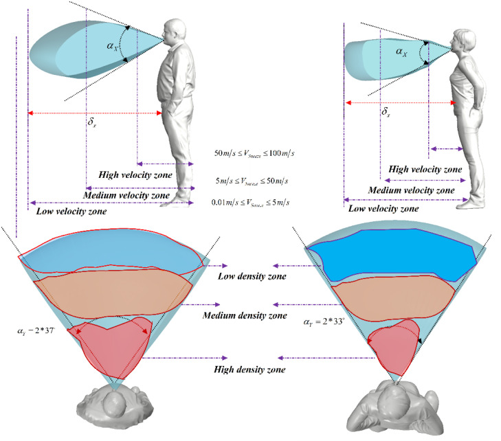
The distribution of droplets and angle of separation for different genders, based on the image processing method.

6 Results and discussion

6.1 Sneezing dynamics

Sneezing is a fully automated process and a natural reaction to remove any contaminants from the lungs. This process travels as a pressure wave from the lungs to the mouth (Li et al., 2020, Burke, 2012, Kitta et al., 2016). This high-pressure flow, once expelled from human mouse and nose, distributes saliva in the form of droplets in the environment. The generated flow changes the size and diameter of these droplets. Modeling of these changes during the sneezing process is one of the most important features of the current work. Previous studies often used particle distribution models based on the distribution of the spherical particles (Han et al., 2013, Dan et al., 2019, Song et al., 2020, Jiang et al., 2018). This prevents examination of the changes in droplet diameter during the sneezing process. Further, since movement within the air-fluid causes deformation of the droplets, the drag force caused by the deformation is not constant and this has a significant effect on the droplet distribution.

Fig. 6 shows a typical view of the process of breaking droplets during the sneezing process in the vicinity of human mouth. This analysis was conducted by image processing applied on the LES results. It shows that large droplets fall into small particles within a short distance. It also shows that the concentration of saliva in the unit volume of the densely packed area is much higher than other areas. Fig. 6 further indicates that the break and splitting of large droplets due to the internal forces and drag forces reduce the concentration in the constant volume. This, in turn, leads to the expansion of the contaminated space with sneezing droplets. The spread of virus in the process of sneezing depends on various parameters such as speed and direction, as well as the virus concentration in saliva. Further, it has been shown that the physical properties of saliva varies amongst different people (Ericsson and Stjernström, 1951, Briedis et al., 1980).

Fig. 6

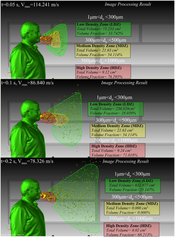
Distribution and breakup of the saliva droplets in the vicinity of the sneezing person (T_inf=25°C, Velocity=90 m/s, number of droplets = 5,000,000, t = 0.1 s).

The statistics of droplet diameter is an essential outcome of the current analysis. It is already evident that there exists a correlation between the droplet diameter and the possibility of infection transmission (Chen, 2020, Kotb and Khalil, 2020, Busco et al., 2020, Li et al., 2020). The changes in diameter depends on the evaporation rate, flow field and the physical properties of saliva. Fig. 7 shows the statistical distribution of droplets based on the average diameter at two different instances of time. The results clearly show that the droplet diameter is strongly time dependent. Changes in the droplet diameter directly influence the droplet distribution. As such, there is a direct relation between droplet diameter and deposition rate. Also, increasing the rate of evaporation may help reducing the concentration of droplets near the sneezing person. Particles with diameters of 1–250 micrometers are more likely to become suspended. These particles are not transported by air flow to far distances from the sneezing person.

Fig. 7

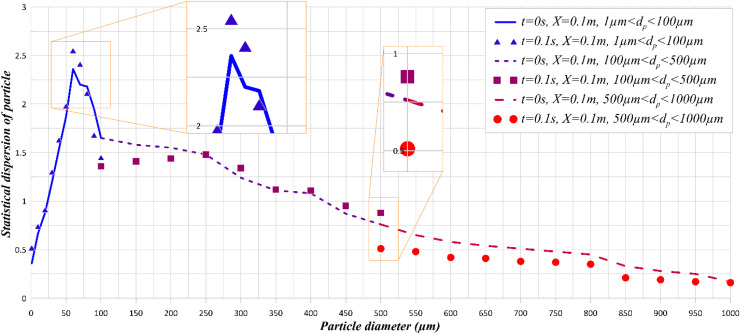
Frequency of droplest diameter at X = 2 m and for T_inf= 25°C.

As shown in Fig. 7, it is also clear that the distribution of particles in the transversal direction within the range of 1–100 µm is the greatest. The issue of sneezing and its spread in the investigated environment (inside the bus) has some unique features. First, the infected person sneezes at the end of the bus and the droplets are spread out by natural dispersion as well as the air flow set by the ventilation system. Second, the ambient temperature influences the particle density by altering the evaporation rate. Further, it has been shown that the evaporation rate has an inverse relationship with the droplet diameter and decreases with increasing the droplet diameter (Hasan, 2020). Fig. 7 further shows the effects of temporal changes on different droplet diameters. It is important to note that during the sneezing process, the time and size of the droplets play a major role in the spread of the virus.

6.2 Droplet dispersion in the bus-CFD approach

In general, there are two important factors dominating the probability of infection: exposure time and concentration of virus (Ueba, 1978, Gerba, 1984, Jang et al., 2014). Sneezing process involves a wide range of droplet diameter with different velocity. According to the weight and diameter, each particle has a specific deposition velocity. It follows that the spatial analysis of particle diameter and concentration can help assessing the risk of infection.

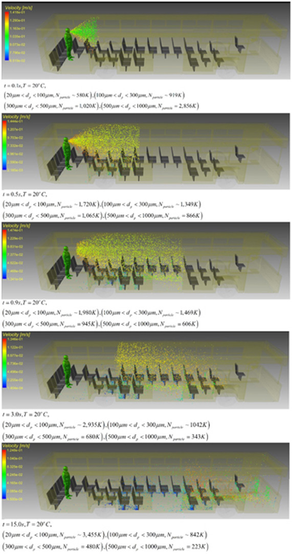
Fig. 8 shows the distribution of droplets within the range of two meters from the person. The classification of regions in Fig. 8a is on the basis of the downward velocity of the droplets which drives the sedimentation process. A volume of 2 m³ was considered in front of the sneezing person and a series of image processing techniques were employed to identify the droplet velocity. This led to identification of three spatial regions. In the green region, the ensemble average of the downward velocity of droplets is less than 0.001 m/s. This quantity increases to 0.1 m/s and 0.5 m/s in the blue and brown regions. As shown in Fig. 8a, the affected area of sneezing droplets can generally be divided into three parts based on concentrations. In this figure, drawn along the vertical and horizontal axis of the bus geometry, it is clear that the sneezing person disperses a different percentage of droplets in each area. The path lines have been shown for a selected number of droplets. Most of droplets in the low-density region are those with diameters between 1 and 25 µm, while the droplets with a diameter of 113–225 µm are most common in the medium density section. As stated previously, the deposition rate of every droplet is directly related to the diameter, therefore it is expected that smaller diameter droplets would be dispersed farther away from the sneezing person. It is observed that in the area with high density, particles of 510–700 µm are most common. The deposition rate of the particles and the time they remain suspended depend directly on the particle diameter. Regardless of the resultant forces, the droplet diameter has a direct effect on the deposition time. Also, due to the changes in diameter along the longitudinal direction of the bus, it can be stated that the droplet deposition time increases directly. Expectedly, heavy droplets deposit at a faster rate than those with a smaller mass.

Fig. 8

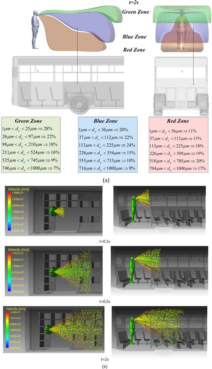
Image processing detection of the distribution of selected droplets at t = 0.1 s, t = 0.5 s and t = 2 s a) side view b) top view (T_inf=25°C).

Fig. 8b shows the distribution of droplets from the top view. It is clear that the pattern of transverse distribution varies according to the location of the individual as well as other environmental parameters. Heavy particles are scattered quickly and in front of the sneezing person. Due to their high mass and inertia, these particles have less deviation from the axial direction of sneezing. This figure further shows that in the areas with low density (green) particles are more prone to be affected by the suction and ventilation system of the bus.

Fig. 8b, depicts the top view of droplet distribution in the bus. It is inferred from this figure that the cross-section of the particle transport may change the areas of accumulation of heavy particles. The diffusion environment varies based on the position in the three-dimensional space, the distance between the droplet and the sneezing location for different models. The results further indicate that according to the particle mass, the path of a particle can be different. Also, by comparing Figs. 8a and b, it is clear that the process of transfer and deposition of particles is strongly dependent on the time and environmental conditions. The process of distributing the sneezing particles in the bus is statistically affected by the environmental conditions.

The deposition process and distribution of droplets were studied computationally up to 2 m from the sneezing person. Fig. 9 shows the contours of droplet concentration drawn on three planes at the distances of 0.5, 1 and 2 m from the sneezing person. In order to compare the droplet concentration, Fig. 9 is based on the percentage of droplets per unit volume (number of particles or droplets in standard control volume by considering the evaporated mass of droplets).

c o n c e n t r a t i o n (%) = (\frac{n u m b e r o f p a r t i c l e (s e l e c t e d r a n g e)}{n u m b e r o f p a r t i c l e (s e l e c t e d r a n g e) i n t = 0.1 s i n C . V c l o s e t o t h e f a c e})

(26)

Fig. 9

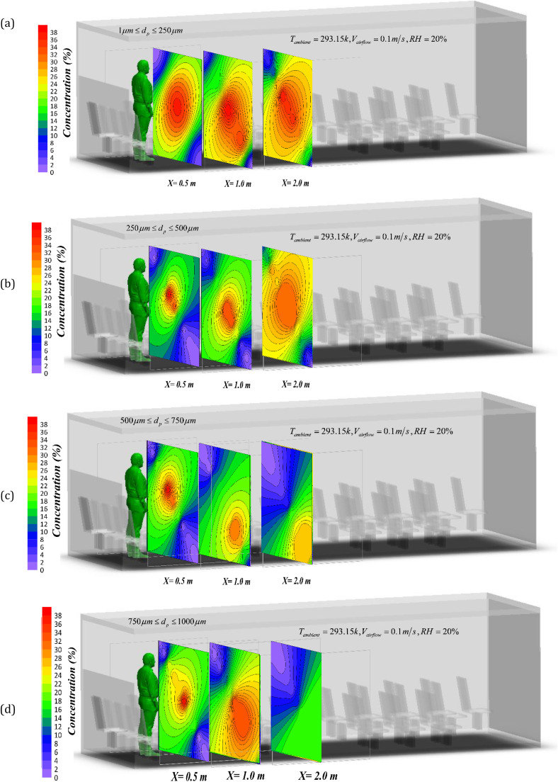
Spatial distribution of the droplet concentration in 2 m distance from the sneezing person for a) 1–250 µm, b) 250–500 µm, c) 500–750 µm, d) 750–1000 µm droplet diameter at t = 5 s after sneezing.

The results show that the droplet diffusion is directly related to the droplet size. It is known that increasing the diameter of the droplets modifies the distribution model and alters the maximum deposition location. Fig. 9 shows that for the droplets with diameters between 1 and 250 µm, there exists a very small amount of sedimentation. That is to say that the droplets of this size practically do not sediment and remain suspended and therefore can be easily transferred along the bus. These droplets are the primary suspect of the infection parameter. As an important point, Fig. 9 further shows that the ventilation system can reduce the droplet concentration by removing the droplets. Some of these droplets, with the diameters between 250 and 500 µm, may deposit. Other droplets can be still transferred along the bus and contribute to transmission of the virus.

By increasing the droplet diameter, the deposition rate is expected to increase. According to Fig. 10, the droplets with diameters of 500–750 µm can deposit quickly within a short distance from the sneezing person. The results show that for this range of droplet diameter, there is a large concentration gradient along the bus. Overall, the simulations indicate that the droplets with diameters of 1–250 µm have the highest diffusion speed amongst all generated droplets. This is because of their small size and their ability to be suspended in air. According to Fig. 10, for the droplets with the diameter of 1–250 µm at a distance of two meters, the velocity changes are greater than those of other droplets. Also, the results in Fig. 10 show that with increasing the diameter of the droplets, their average velocity decreases by a factor three, which clearly shows the importance of spreading the droplets with small diameters.

Fig. 10

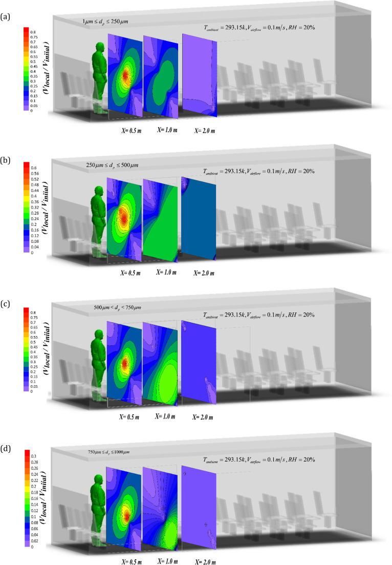
Non-dimensional velocity for the droplets distribution within 2 m distance from the sneezing person for a) 1–250 µm, b) 250–500 µm, c) 500–750 µm, d) 750–1000 µm droplet diameter at t = 5 s after sneezing.

6.3 Droplet dispersion in the bus-AI approach

The last section demonstrated that the computational model can provide an insight into the spread of virus in the selected environment (bus). Nonetheless, the computational burden of the model poses a serious practical issue. Rapid computation for risk assessment purposes is almost impossible and therefore alternative approaches should be sought for the prediction of particle distribution. The use of AI can reduce the computational cost of the analysis and increase the processing speed up to almost 100 times. Here, the computationally generated data are used to train an AI tool (see Section 4) that predicts the temporal and spatial evolution of the particle distribution in the bus. In Fig. 11, the results obtained from the AI model and those produced through numerical simulations are presented for four different areas. A comparison between the two sets of data confirms the accuracy of the developed AI tool to predict the droplet distribution. The excellent agreement between the computationally and AI generated data means that artificial intelligence can predict the concentration in the entire volume of the bus. As shown in Fig. 10, these values are for the middle plane of the bus and the midline on this plane. It is important to note that with increasing the computational accuracy in region 1, fewer changes for the data obtained from artificial intelligence are encountered.

Fig. 11

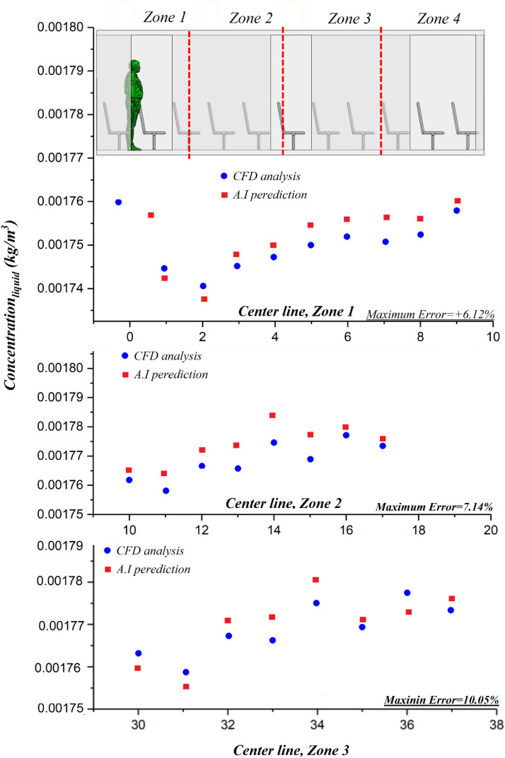
Comparison between the CFD results and AI predictions at different locations along the bus.

In Fig. 12, the concentration of particles has been plotted based on their diameter distribution in the whole volume of the bus over 9 different parallel planes with increasing distance from the sneezing person. It is recalled that computational modeling was performed only for the first two meters away from the sneezing person and the rest of the domain was predicted by the AI tool. In keeping with the computational result, the AI results show that smaller diameter particles can propagate widely throughout the bus. As farther distance is taken from the sneezing person, a decrease in the concentration of particles and a gradual deposition of particles in different parts are observed. The data presented in this figure are based on the Aceh emission analysis model at the distance of two meters. In producing those data, the maximum particle density was plotted on each plane for 10 s. Also, the presence of ventilation in the bus and the upper part of the passengers’ heads can change the pattern of the particle distribution. It is further observed that the particles with small diameters are readily transported throughout the bus. Also, heavy particles evaporate and turn into smaller particles. The presence of flow obstacles such as passenger seats impart a major effect on the distribution and suspension of particles as well as sedimentation of the settling particles. This is because the air flow is very small in between the seats. Thus, the sedimentation model and the deposition of particles are modified in the space between the seats. The results show that artificial intelligence has the capability of predicting the temporal and spatial distribution of particles in the complex and highly varying environment of the bus. Since AI analysis is much faster (around 100 times) than the corresponding computational analysis, it can be used in practice to evaluate the spread of droplets and the associated risk of infection. An overall view of the temporal spread of droplets within the bus can be found in the companion animation file. In there, the data on the first 2 m from the sneezing passenger have been extracted from the CFD analysis and the spread of droplets in the rest of the bus was predicted by the AI tool.

Fig. 12

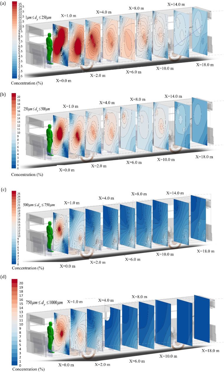
Distribution of the droplet concentration in 18 m distance from the sneezing person for a) 1–250 µm, b) 250–500 µm, c) 500–750 µm, d) 750–1000 µm droplet diameter at t = 10 s after sneezing.

7 Conclusions

Protection against COVID-19 and establishment of relevant risk assessment schemes are currently central to the health and wellbeing of the society. Understanding the patterns of virus spread and their pertinent parameters are amongst the key issues raised in the recent months. Importantly, there is a pressing need for the quick assessment of transmission risk in indoor environments with large occupancy. In particular, public transport has been identified as one of the main routes to virus transmission. This poses a major challenge on the conventional simulations based on computational fluid dynamics, as the required computational time makes them impractical for risk assessment. To address this issue, an attempt was made to provide a novel approach to the prediction of droplet distributions set by sneezing of an infected person in a bus. This was based on the high fidelity computation of the droplets formation during the sneezing process followed by the droplets dispersion in the domain up to 2 m away from the sneezing person. The processes of droplets formation and spread were modeled through applying the volume of fluid and LES methodologies to the person’s mouth and the immediate surroundings. The resultant computational data were then used to develop an AI-based tool capable of predicting the evolution of droplet distribution in the entire volume of the bus. It was shown that while the AI-based approach reduces the computational time most significantly (~100 times), it offers an excellent accuracy. Hence, the developed combined scheme on the basis of CFD and AI is deemed suitable for practical risk assessments.

In addition to this, the following physical outcomes emerged from this work.

1.The boundary conditions have substantial effects on the droplet dispersion. The ambient velocity and initial speed of droplets can widen the septic zone.

2.The droplet diameter dominates the dispersion process. The droplets with smaller diameters (less than 250 µm) are very likely to remain suspended in air and thus be transferred to other parts of the environment.

3.The results indicate that about 59% of the initial droplet will be deposited in the first 2 m away from the sneezing person. The droplets with diameters between 500 and 1000 µm are most likely to fall and hit the ground within this distance.

4.The concentration of droplets could decline to 87% in the first 3 m. Nonetheless, this process is heavily affected by the ambient temperature and airflow velocity.

CRediT authorship contribution statement

Mehrdad Masgarpour: Conceptualization, Software, Validation, Formal analysis, Writing - original draft. Javad Mohebbi Najm Abad: Software, Data curation, Investigation. Asool Alizadeh: Investigation, Project administration. Somchai Wongwises: Resources, Supervision. Mohammadhossein Doranehgard: Writing - review & editing. Saeidreza Ghaderi: Writing - original draft. Nader Karimi: Conceptualization, Supervision, Project administration, Writing - review & editing.

Declaration of Competing Interest

The authors declare that they have no known competing financial interests or personal relationships that could have appeared to influence the work reported in this paper.

References

Abuhegazy

, Talaat

, Anderoglu

, Poroseva

S.V.

. Numerical investigation of aerosol transport in a classroom with relevance to COVID-19.

103311

Alizadeh

. A machine learning approach to predicting the heat convection and thermodynamics of an external flow of hybrid nanofluid.

Alizadeh

, Mohebbi Najm Abad

, Fattahi

, Alhajri

, Karimi

. Application of machine learning to investigation of heat and mass transfer over a cylinder surrounded by porous media-the radial basic function network.

Briedis

, Moutrie

, Balmer

. A study of the shear viscosity of human whole saliva.

Burke

. Why do we sneeze?.

Busco

, Yang

S.R.

, Seo

, Hassan

Y.A.

. Sneezing and asymptomatic virus transmission.

073309

Chabert

, Dorfman

K.D.

, Viovy

J.L.

. Droplet fusion by alternating current (AC) field electrocoalescence in microchannels.

Chaudhuri

, Basu

, Kabi

, Unni

V.R.

, Saha

. Modeling the role of respiratory droplets in Covid-19 type pandemics.

063309

Chen

L.-D.

. Effects of ambient temperature and humidity on droplet lifetime - a perspective of exhalation sneeze droplets with COVID-19 virus transmission.

113568

Christodoulou

, Karimi

, Cammarano

, Paul

, Navarro-Martinez

. State prediction of an entropy wave advecting through a turbulent channel flow.

Crowe

C.T.

Multiphase Flows with Droplets and Particles

CRC Press

Dan

H.-C.

, Zou

Z.M.

, Chen

J.Q.

, Peng

A.P.

. DEM-aided method for predicting the hydraulic properties with particle-size distribution of porous media.

Diwan

S.S.

, Ravichandran

, Govindarajan

, Narasimha

. Understanding transmission dynamics of COVID-19-type infections by direct numerical simulations of cough/sneeze flows.

Jun

, Xu

Yong

. Hierarchical deep neural network for multivariate regression.

Dutta

, Spence

, Wei

, Dhapare

, Hindle

, Longest

P.W.

. CFD guided optimization of nose-to-lung aerosol delivery in adults: effects of inhalation waveforms and synchronized aerosol delivery.

Enserink

, Kupferschmidt

With COVID-19, Modeling Takes on Life and Death Importance

American Association for the Advancement of Science

Ericsson

, Stjernström

. Saliva viscosity measurements.

Gerba

C.P.

. Applied and theoretical aspects of virus adsorption to surfaces.

Gupta

, Lin

C.H.

, Chen

. Flow dynamics and characterization of a cough.

Hamey, P., The evaporation of airborne droplets. 1982.

Han

, Weng

, Huang

. Characterizations of particle size distribution of the droplets exhaled by sneeze.

20130560

Hasan

. Tracking the flu virus in a room mechanical ventilation using CFD tools and effective disinfection of an HVAC system.

2050019

Hassani

, Khorramymehr

. In silico investigation of sneezing in a full real human upper airway using computational fluid dynamics method.

Hendry

J.R.

, Lee

J.G.

, Battrum

M.J.

. CFD model of fluid flow and particle deposition during cryogenic condensation.

Huang

, Zhu

, Zhou

, Gou

, Yu

, Li

, Tong

, Yang

. Role of CFD based in silico modelling in establishing an in vitro-in vivo correlation of aerosol deposition in the respiratory tract.

Ivanov

, Mijorski

. Assessment of transient CFD techniques for virtual thermal manikins’ breathing simulations.

Ivorra

, Ferrández

M.R.

, Vela-Pérez

, Ramos

A.M.

. Mathematical modeling of the spread of the coronavirus disease 2019 (COVID-19) taking into account the undetected infections. The case of China.

105303

Jang

, Lee

, So

, Lee

, Yun

, Lee

, Choe

. Evaluation of changes induced by temperature, contact time, and surface in the efficacies of disinfectants against avian influenza virus.

Jiang

M.D.

, Yang

Z.X.

, Barreto

, Xie

Y.H.

. The influence of particle-size distribution on critical state behavior of spherical and non-spherical particle assemblies.

Kim

Y.H.

, Tong

Z.B.

, Chan

H.K.

, Yang

R.Y.

. CFD modelling of air and particle flows in different airway models.

Kitta

, Yoshikawa

, Kawamorita

, de Groat

W.C.

, Nonomura

, Yoshimura

. The effect of ovariectomy on urethral continence mechanisms during sneeze reflex in middle‐aged versus young adult rats.

Kolev

N.I.

, Kolev

N.I.

Multiphase Flow Dynamics: Fundamentals

Springer

Kotb

, Khalil

E.E.

. Impact of sneezed and coughed droplets produced from a moving passenger on other passengers inside aircraft cabins.

, Leong

F.Y.

, Xu

, Ge

, Kang

C.W.

, Lim

K.H.

. Dispersion of evaporating cough droplets in tropical outdoor environment.

113301

Link

D.R.

, Grasland-Mongrain

, Duri

, Sarrazin

, Cheng

, Cristobal

, Marquez

, Weitz

D.A.

. Electric control of droplets in microfluidic devices.

, Lu

. CFD investigation on particle deposition in aligned and staggered ribbed duct air flows.

Meccariello, G. and O. Gallo, What ENT doctors should know about COVID-19 contagion risks. Authorea Preprints, 2020.

Mohebbi Najm Abad

, Alizadeh

, Fattahi

, Doranehgard

M.H.

, Alhajri

, Karimi

. Analysis of transport processes in a reacting flow of hybrid nanofluid around a bluff-body embedded in porous media using artificial neural network and particle swarm optimization.

113492

, Wang

, Zhai

, Shang

, Zhao

, Yin

. Unsteady CFD simulation on ash particle deposition and removal characteristics in tube banks: focusing on particle diameter, flow velocity, and temperature.

Niu

, Gulati

, Edel

J.B.

, deMello

A.J.

. Pillar-induced droplet merging in microfluidic circuits.

Pendar

M.-R.

, Páscoa

J.C.

. Numerical modeling of the distribution of virus carrying saliva droplets during sneeze and cough.

083305

Ranz

, Marshall

W.R.

. Evaporation from drops.

Rockett

R.J.

, Arnott

, Lam

, Sadsad

, Timms

, Gray

K.A.

, Eden

J.S.

, Chang

, Gall

, Draper

, Sim

E.M.

, Bachmann

N.L.

, Carter

, Basile

, Byun

, O’Sullivan

M.V.

, Chen

S.C.A.

, Maddocks

, Sorrell

T.C.

, Dwyer

D.E.

, Holmes

E.C.

, Kok

, Prokopenko

, Sintchenko

. Revealing COVID-19 transmission in Australia by SARS-CoV-2 genome sequencing and agent-based modeling.

Schmidt-Hieber

Johannes

. Nonparametric regression using deep neural networks with ReLU activation function.

Seyfi

, Mirzayi

, Seyyedbagheri

. CFD modeling of black powder particles deposition in 3D 90-degree bend of natural gas pipelines.

103330

Singh

R.K.

, Tripathi

S.N.

. Application of national aerosol facility (NAF) in designing of a ventilation system for isolation rooms to minimize interpersonal exposure of sneezing/coughing.

Song

, Wei

, Sun

, Chen

. Experimental and CFD study of particle deposition on the outer surface of vortex finder of a cyclone separator.

Song

, Rong

, Dong

, Liu

, Le Clech

, Shen

. Particle-scale modelling of fluid velocity distribution near the particles surface in sand filtration.

115758

Ueba

. Respiratory syncytial virus. I. concentration and purification of the infectious virus.

Verma

, Dhanak

, Frankenfield

. Visualizing droplet dispersal for face shields and masks with exhalation valves.

091701

Vuorinen

, Aarnio

, Alava

, Alopaeus

, Atanasova

, Auvinen

, Balasubramanian

, Bordbar

, Erästö

, Grande

, Hayward

, Hellsten

, Hostikka

, Hokkanen

, Kaario

, Karvinen

, Kivistö

, Korhonen

, Kosonen

, Kuusela

, Lestinen

, Laurila

, Nieminen

H.J.

, Peltonen

, Pokki

, Puisto

, Råback

, Salmenjoki

, Sironen

, Österberg

. Modelling aerosol transport and virus exposure with numerical simulations in relation to SARS-CoV-2 transmission by inhalation indoors.

104866

Yang

, Ingham

, Ma

, Zhou

, Pourkashanian

. Understanding the ash deposition formation in Zhundong lignite combustion through dynamic CFD modelling analysis.

Yeoh, G.H. and J. Tu, Computational techniques for multiphase flows. 2019: Butterworth-Heinemann.

Acknowledgment

The first author (M. Mesgarpour) acknowledges Postdoctoral Fellowship from KMUTT. S. Wongwises acknowledges the support provided by the "Research Chair Grant "National Science and Technology Development Agency (NSTDA), and King Mongkut's University of Technology Thonburi through the "KMUTT 55th Anniversary Commemorative Fluid. N. Karimi acknowledges the financial support by the Engineering and Physical Science Research Council, UK, through the grant number EP/V036777/1 Risk Evaluation Fast Intelligent Tool (RELIANT) for COVID 19.

Appendix A Supplementary data associated with this article can be found in the online version at doi:10.1016/j.jhazmat.2021.125358.