Network-level time series of a temporal network

To characterize temporal correlations in temporal networks, we apply the multiscale entropy (MSE) method [49, 50] to the network-level time series of empirical face-to-face interaction datasets. As for the network-level time series, we first consider a time series for the number of interactions between individuals or activated links, as it is the simplest quantity measuring the overall interaction patterns of the temporal network. We also study the time series of the number of newly activated links or links that are activated for the first time. This quantity may capture the evolutionary dynamics of the network topology because the first activation of a link can be interpreted as the creation of the link.

We introduce notations for the temporal network with N nodes, K links, and the total number of activations over all links W during the observation period of T. Each link i (i = 1, …, K) at a time step t (t = 1, …, T) can be either in an active state (interaction) or in an inactive state (no interaction), which are denoted by A_i(t) = 1 and 0, respectively. The number of activated links at the time step t, denoted by W(t), is given as $$ W\left(t\right)={\sum }_{i=1}^K{A}_i\left(t\right)$$. Note that a weight of the link i can be obtained by $$ w_i\equiv {\sum }_{t=1}^T{A}_i\left(t\right)$$. We also denote the number of newly activated links at the time step t by K(t). By definition K(t) ≤ W(t). The time series of K(t) and W(t) are written as {K(t)} and {W(t)}, respectively, where $$ {\sum }_{t=1}^{T}K\left(t\right)=K$$ and $$ {\sum }_{t=1}^{T}W\left(t\right)=W$$. Fig 1 shows an example of {K(t)} and {W(t)} for the temporal network with N = 5, K = 8, W = 12, and T = 9. The time-resolved and time-aggregated representations of the temporal network are shown in the top panels, while {K(t)} and {W(t)} are presented in the bottom panel.

Fig 1

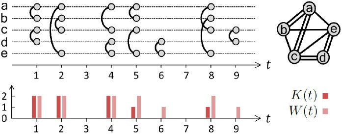
An example of a temporal network in discrete time.

The time-resolved and time-aggregated representations of the network (top) and the network-level time series of {K(t)} and {W(t)} (bottom). Here W(t) and K(t) denote the number of activated links and the number of newly activated links at the time step t, respectively.

Activity patterns in many temporal network datasets are known to be non-Poissonian or bursty [7], implying the existence of temporal correlations or memory effects, which are often found in multiple timescales. For characterizing the activity patterns with multiscale temporal correlations, we adopt the MSE method [49, 50]. It is because the face-to-face interaction datasets to be studied in our work have relatively short observation periods and the MSE method has been known to be less dependent on the time series length such as in physiological systems [49].

Multiscale entropy

We present a brief review of the multiscale entropy (MSE) method [49, 50] for characterizing the time series with multiscale temporal correlations. Here, we describe the MSE method using the notations and symbols used in Refs. [49, 50].

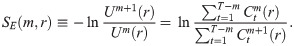
We first define the sample entropy [61]. Let us consider a univariate discrete time series {x_t} for t = 1, …, T, from which we get T − m vectors of length m, i.e., $$ X_t^m=(x_t,\dots ,x_{t+m-1})$$ for t = 1, …, T − m. For a given vector $$ X_t^m$$, one can calculate the probability $$ C_t^m\left(r\right)$$ that a random vector $$ X_{t^{\prime }}^m$$ for t′ ≠ t lies within a distance r from $$ X_t^m$$, namely, satisfying max{|x_t+s − x_t′+s|}_{s = 0, …, m − 1} ≤ r. Then the average of $$ C_t^m\left(r\right)$$ over t is denoted by $$ U^m\left(r\right)\equiv {(T-m)}^{-1}{\sum }_{t=1}^{T-m}{C}_t^m\left(r\right)$$. Similarly, one can get T − m vectors of length m + 1, denoted by $$ X_t^{m+1}$$, from which $$ C_t^{m+1}\left(r\right)$$ and U^m+1(r) are respectively calculated. Using U^m(r) and U^m+1(r) one defines the sample entropy, denoted by S_E(m, r), as follows:

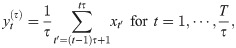
To analyze the time series with multiscale temporal correlations by means of the sample entropy S_E, Costa et al. proposed the MSE method [49] by incorporating a coarse-graining procedure. For a given time series {x_t} for t = 1, …, T and the scale factor τ, the coarse-grained time series $$ \left\{y_t^{\left(\tau \right)}\right\}$$ for t = 1, …, T/τ is constructed by averaging the elements in {x_t} within non-overlapping time windows of size τ such that

Fig 2

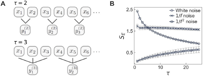
Multiscale entropy (MSE) method.

(A) A schematic illustration of coarse-graining procedure of the time series {x_t} for t = 1, …, T with the scale factor τ = 2 (top) and 3 (bottom). (B) Numerical results of the MSE method applied to the white noise, the 1/f noise, and the 1/f² noise. Each value of S_E is averaged over 10 time series with T = 3 × 10⁴, and the error bar denotes its standard deviation.

For the demonstration of the MSE method, we apply this method to three kinds of time series, i.e., white noise and 1/f noise as in Refs. [49, 50], and 1/f² noise as in Ref. [62]. Here we generate a time series for white noise using random numbers that are drawn from a normal distribution with zero mean and variance of one. To generate a time series for 1/f noise we use the Voss-McCartney algorithm [63, 64]. Finally we generate a time series for 1/f² noise using a Brown noise generator [65], which is essentially the temporal integration of white noise. The white noise is uncorrelated time series, while 1/f and 1/f² noises are non-stationary as well as have strong temporal correlations with infinite memory and long-term memory in terms of decaying behaviors of autocorrelation functions, respectively [66, 67]. The results of the MSE method for these time series are presented in Fig 2(B). In the case of the white noise, S_E monotonically decreases as τ increases, whereas S_E remains almost constant for the 1/f noise, and S_E monotonically increases for the 1/f² noise. The monotonically decreasing S_E for the white noise implies that the noisy, random behavior tends to be averaged out for the larger scale factor. In contrast, the overall constant S_E for the 1/f noise must be due to the temporal self-similarity of 1/f noise. Finally, the monotonically increasing S_E for the 1/f² noise indicates that coarse-graining by the larger scale factor enhances the fluctuation of time series, hence makes the time series look more random.

Datasets

We consider six empirical face-to-face interaction datasets provided by the SocioPatterns project [68]: a primary school dataset for 2 days, a hospital dataset for 5 days from 6 a.m. to 8 p.m. for each day, a workplace dataset for 10 days, a high school dataset for 4 days in 2011, a high school dataset for 7 days in 2012, and a conference dataset for 3 days. The high school datasets in 2011 and 2012 are denoted as “school (2011)” and “school (2012)”, respectively. Table 1 provides information about the datasets, including the observation period in terms of the number of days and the number of distinct nodes in each dataset. In all datasets, contacts or interactions between individuals were recorded every 20 seconds, defining the unit of the time step in our work.

Table 1

or each dataset, we present the observation period in terms of the number of days, the minimum and maximum numbers of nodes in the daily partition of the dataset (N_min and N_max), and the number of distinct nodes in the entire dataset (N_tot), respectively.

Information about the datasets.

Dataset	Primary school	Hospital	Workplace	School (2011)	School (2012)	Conference
days	2	5	10	4	7	3
Nmin	236	40	59	112	145	97
Nmax	238	50	72	121	158	102
Ntot	242	75	92	126	180	113

Topological properties of time-aggregated networks

We first investigate the basic topological properties of time-aggregated networks. We obtain the time-aggregated network for each day of each dataset to get degree and weight distributions, where the degree k means the number of neighbors. These daily distributions are averaged for each dataset to get the averaged P(k) and P(w), as shown in Fig 3. We observe that P(k)s show increasing and then decreasing behaviors, while being mostly right-skewed, except for the case with the primary school. P(k) for the primary school shows both large average and large variance of degrees. The weight distributions P(w) are found to show the similar heavy-tailed behaviors across all datasets. We conclude that the topological structures of time-aggregated networks of six datasets are qualitatively similar to each other.

Fig 3

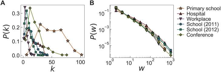
Degree distributions P(k) and weight distributions P(w) for empirical datasets.

(A) P(k) and (B) P(w) of time-aggregated networks for six face-to-face interaction datasets, i.e., for the primary school (✰), hospital (△), workplace (▽), school (2011) (○), school (2012) (□), and conference (◊). P(k)s are linearly binned, while P(w)s are logarithmically binned.

Multiscale entropy analysis on empirical datasets

Next, we apply the MSE method to the time series {K(t)} and {W(t)} derived from the above mentioned datasets. For each day of each dataset, we calculate the sample entropy S_E for the coarse-grained time series using the scale factor of τ = 1, …, 100. Then the curves of S_E as a function of τ are averaged over all days for each dataset, denoted by $$ \overline{S_E}$$. The results of $$ \overline{S_E}$$ are presented with the corresponding standard deviations in Fig 4, where the top (bottom) panels show the results for {K(t)} ({W(t)}). From now on we denote $$ \overline{S_E}$$ for {K(t)} and {W(t)} as $$ \overline{S_E^K}$$ and $$ \overline{S_E^W}$$, respectively.

Fig 4

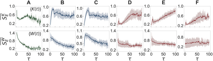
Results of the MSE method for empirical datasets.

Results of the MSE method applied to time series {K(t)} (top panels) and {W(t)} (bottom panels), respectively denoted as $$ \overline{S_E^K}$$ and $$ \overline{S_E^W}$$, of six face-to-face interaction datasets: (A) primary school, (B) hospital, (C) workplace, (D) school (2011), (E) school (2012), and (F) conference. See the main text for details.

According to the behavioral patterns of $$ \overline{S_E^K}$$, the six datasets can be divided into three categories: (i) The primary school dataset shows the overall increasing and then decreasing behavior of $$ \overline{S_E^K}$$, apart from the peak at τ = 1 [top panel in Fig 4(A)]. Note that the decreasing behavior of $$ \overline{S_E^K}$$ was observed for the white noise in Fig 2(B). (ii) $$ \overline{S_E^K}$$ for hospital and workplace datasets increases quickly and then decreases very slowly or even fluctuates around some constant [top panels in Fig 4(B) and 4(C)]. The behavior that remains almost constant is similar to the result for the 1/f noise in Fig 2(B), implying the long-range temporal correlations. (iii) The other three datasets, i.e., school (2011), school (2012), and conference, show the overall increasing $$ \overline{S_E^K}$$ [top panels in Fig 4(D)–4(F)], indicating that the time series appears to be more complex when looked at in longer timescales. Note that the increasing behavior of $$ \overline{S_E^K}$$ was observed for the 1/f² noise in Fig 2(B), and also the similar increasing behaviors have been reported for neural time series [69–71].

It is remarkable to mention that in all cases we find a peak around at a small value of τ whether the peak is a global maximum (primary school, hospital, and workplace) or a local maximum (school (2011), school (2012), and conference). These peaks may indicate that all time series we analyzed contain random noise of short timescales to some extent, which is however effectively averaged out in the procedure of coarse-graining with larger values of τ.

Results for {W(t)} in the bottom panels of Fig 4 can be better understood by comparing them with those for {K(t)} as W(t) is the sum of K(t) and the number of activated links that have been activated before the time t. The latter kind of activations, corresponding to W(t) − K(t), indeed leads to different behaviors of $$ \overline{S_E^W}$$ than $$ \overline{S_E^K}$$: In the case with the primary school, $$ \overline{S_E^W}$$ overall monotonically decreases, implying that the values of {W(t)} are more uncorrelated with each other than those of {K(t)}. $$ \overline{S_E^W}$$ for the hospital and workplace datasets overall decreases for the almost entire range of τ, implying the long-range correlations in {K(t)} must have been largely destroyed in {W(t)}. Finally, the other three datasets for school (2011), school (2012), and conference show the almost flat behaviors of $$ \overline{S_E^W}$$, similarly to the case with 1/f noise. In sum, we find that the activations observed by W(t) − K(t) tend to weaken the temporal correlations present in {K(t)}.

Heterogeneity level and memory coefficient

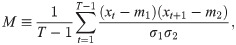
For more detailed understanding of the empirical results by the MSE method, we introduce two quantities for characterizing {K(t)} and {W(t)}: the heterogeneity level H and the memory coefficient M. These quantities are based on the burstiness parameter and memory coefficient that were originally proposed in Ref. [72] for measuring the temporal correlations in the point processes in terms of interevent times. In our work, instead of interevent times, we analyze the values of time series of {x_t} for t = 1, …, T. To measure how broad the distribution of values of x_t is compared to their mean, we calculate the mean and standard deviation of the values of x_t, respectively denoted by m_x and σ_x, to define the heterogeneity level H as follows:

We calculate the values of H and M for {K(t)} and {W(t)} for each day of each dataset. These values are plotted in the (M, H)-spaces as shown in Fig 5. In the case with {K(t)}, we clearly find three clusters of points: (i) The primary school dataset is characterized by the smallest values of H (≈0.1) and the largest values of M (≈0.8), implying that the values of the time series are relatively homogeneous, while they are strongly correlated with each other. (ii) The hospital and workplace datasets show the large values of H (0.4 ≲ H ≲ 0.7) and the small values of M (0 ≲ M ≲ 0.2). It means that the values of the time series are highly heterogeneous, but showing with relatively weak correlations between them. (iii) The other three datasets, i.e., school (2011), school (2012), and conference, show large values of both H and M such that the values of the time series are highly heterogeneous as well as strongly correlated with each other. From the results for {W(t)}, we can observe three clusters similarly to those for {K(t)}, apart from the observation that the values of H (M) are overall much smaller (larger) than those of {K(t)}.

Fig 5

Scatter plot of values of H and M for empirical datasets.

H in Eq (3) and M in Eq (4) in the (M, H)-space for time series (A) {K(t)} and (B) {W(t)} are presented using the same datasets analyzed in Fig 4.

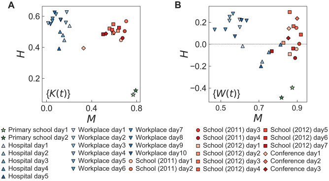
We remark that three clusters identified in the (M, H)-spaces one-to-one correspond to three different behavioral patterns of S_E as a function of τ as discussed above. From such a correspondence one can guess that heterogeneous values of the time series, i.e., large H, are necessary to show the non-decreasing behaviors of S_E. Further, the increasing S_E could additionally require strong positive correlations between consecutive values of the time series.

Interestingly, the datasets in each cluster turn out to share similar social conditions either enhancing or suppressing interactions between individuals. In particular, we focus on the temporal behaviors of such conditions or environmental changes. The participants in the primary school dataset could have break times but only three times including lunch per day [5], while in the high school and conference cases, the interaction between participants were affected by scheduled programs with several breaks [73, 74]. During the breaks participants have chances to introduce each other or strengthen their existing relations, while such interactions can be relatively suppressed for the rest of the observation periods. Unlike schools and conference, there were no constrained schedules for the participants in the hospital and workplace datasets [75, 76]. Generally speaking, the environmental changes can obviously influence the evolution of temporal networks, yet the effects of environmental changes on the evolution of temporal networks are far from being fully understood. To explore such effects, in the following Section we will devise and study a temporal network model that qualitatively reproduces the observed patterns by incorporating the environmental changes.

Modeling a periodic time series

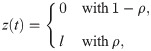
We devise a model for generating a periodic time series {z(t)} for t = 1, …, T, whose values are determined by both the external and internal factors. Considering the fact that the value of the time series of our interest is not always positive in the empirical analysis, we introduce the probability of having a positive z(t), which is denoted by ρ (0 < ρ < 1). Then one can write

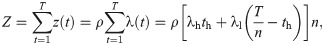
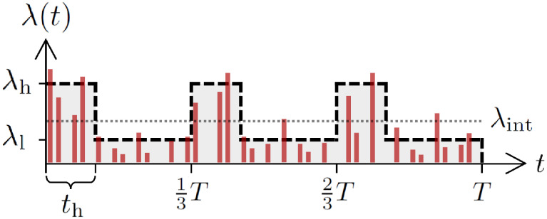
For simplicity, we assume that λ(t) has only two levels of activity, i.e., λ_h and λ_l (λ_h ≥ λ_l). To be precise, the total period T is divided into n intervals. Each interval of length T/n starts with a high activity period of length t_h, for which λ(t) = λ_h. This is followed by a low activity period of length T/n − t_h, for which λ(t) = λ_l. Note that t_h ≤ T/n. In Fig 6 we present an example of λ(t) for the case with n = 3. The sum of z(t) over the entire period of T is assumed to be given as a control parameter Z, namely,

Fig 6

An illustration of the model for generating a periodic time series.

The periodic time series {z(t)} for t = 1, …, T (red vertical lines) is generated using Eqs (5) and (6), where the time-varying parameter λ(t) in Eq (6) (thick dashed curve) is shaped by three parameters, i.e., λ_h, λ_l, and t_h, in the case with n = 3. The horizontal dotted line for λ_int is plotted for comparison. See the main text for details.

For each combination of λ_h/λ_l and t_h, we generate 10³ time series {z(t)} with fixed values of Z = 1000, T = 2000, ρ = 0.2, and n = 5. The multiscale entropy (MSE) method is applied to each time series to get the averaged curve of $$ \overline{S_E}$$ as a function of the scale factor τ, as shown in Fig 7. In the case without external effect, i.e., λ_h/λ_l = 1, we observe the overall decreasing behavior of $$ \overline{S_E}$$, which was observed in the white noise [Fig 2(B)]. As expected, t_h has no effects on the results. As the periodic external effect gets stronger with the larger values of λ_h/λ_l, we find overall flat or even increasing behaviors of $$ \overline{S_E}$$, as depicted in Fig 7(B) and 7(C). Note that the overall flat behavior of $$ \overline{S_E}$$ for λ_h/λ_l = 3 and t_h = 100 was observed in the analysis of 1/f noise [Fig 2(B)]. Furthermore, it turns out that as t_h increases from 100, the range of τ for the flat or increasing $$ \overline{S_E}$$ shrinks and it is followed by the decreasing $$ \overline{S_E}$$ for the large τ regime.

Fig 7

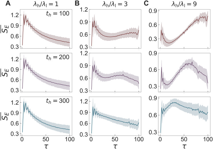
Results of the MSE method for the periodic time series model.

Results of the MSE method applied to the time series {z(t)} using the periodic time series model with Z = 1000, T = 2000, ρ = 0.2, and n = 5 for values of λ_h/λ_l = 1, 3, and 9 (left to right) and t_h, 200, and 300 (top to bottom). For each panel, we have generated 10³ time series to get the averaged curve $$ \overline{S_E}$$ as a function of the scale factor τ.

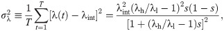
For understanding the effects of t_h on the MSE results in the general case with λ_h/λ_l > 1, we calculate the fluctuation of λ(t) as follows:

Our results for the periodic time series model enable us to get insight into the empirical findings, i.e., decreasing, flat, and/or increasing $$ \overline{S_E}$$, from the temporal network datasets in the previous Section to a large extent.

Modeling temporal networks

Using the periodic time series model in the previous Subsection, we now devise a temporal network model that generates various temporal interaction patterns by considering both external and internal factors. We assume that the periodically changing environment affects not only the topological structure of the network, i.e., newly activated links, but also the activity patterns of links that have previously been activated. The topological structure of the network evolves according to the activity-driven network model [24–30], where each node is activated at its given activity rate to make connections to other nodes. For the activity patterns of previously activated links, we incorporate a preferential activation mechanism for the heavy-tailed weight distributions in Fig 3(B), which is inspired by a preferential attachment mechanism accounting for the power-law degree distributions in scale-free networks [77].

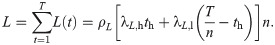
We introduce our temporal network model as follows: At the time step t = 0, we consider a network of N isolated nodes in which each node i is assigned an activity a_i that is drawn from an activity distribution F(a). At each time step t (t = 1, …, T), the number of newly activated links K(t) and the number of activations for previously activated links L(t) are given by assuming that both K(t) and L(t) are affected by the periodically changing environment in a similar way. Therefore, the same periodic time series model in the previous Subsection can be used for both K(t) and L(t) but with different parameter values. Precisely, we use the symbols ρ_K, λ_K,h, and λ_K,l (ρ_L, λ_L,h, and λ_L,l) for modeling K(t) (L(t)), while T, n, and t_h have the same values for K(t) and L(t). These parameters should satisfy the following relations:

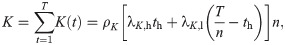
Then K(t) nodes are randomly chosen with probabilities proportional to their activities (a_i). For each chosen node i, we randomly choose another node j that has never been connected to the node i up to the time step t − 1. The link between nodes i and j is created and activated.

For the activation of previously activated links, we first denote by E_t the set of links that have previously been activated up to the time step t − 1. Note that $$ |E_t|={\sum }_{t^{\prime }=1}^{t-1}K\left(t^{\prime }\right)$$. Then L(t) links are randomly chosen from E_t according to the preferential activation mechanism to be activated. By the preferential activation mechanism the more active links in the past are more likely to be activated in the future, which is expected to result in the heavy-tailed weight distributions in the time-aggregated networks. The L(t) links are chosen with probabilities proportional to their accumulated weights up to the time step t − 1, i.e.,

Every activation at the time step t lasts only for one time step before the next time step t + 1 begins. The sum of K(t) and L(t) over the entire period of T is denoted by K and L, respectively, defining the total number of activations across all links W ≡ K + L.

Role of external effect in temporal networks

We generate temporal networks using our temporal network model. Based on the empirical degree distributions in Fig 3(A), all nodes are considered to have the same activity, i.e., a_i = a for i ∈ {1, …, N}. We perform the simulations with the fixed values of N = 100, K = 1000, W = 10000, T = 2000, ρ_K = 0.2, ρ_L = 0.8, and n = 5, but for various combinations of t_h, λ_K,h/λ_K,l, and λ_L,h/λ_L,l. Here the fixed values of parameters are based on the statistics of related quantities derived from datasets except for n. As the choice of n is not obvious from some datasets, we have referred to either the number of breaks (in some datasets) or the number of peaks in the time series for the number of interactions (in other datasets). We consider three cases with parameter values of (t_h, λ_K,h/λ_K,l, λ_L,h/λ_L,l) = (200, 3, 1) (“Case 1”), (100, 3, 1) (“Case 2”), and (100, 9, 1.5) (“Case 3”). These cases correspond to three categories identified by the empirical analysis of six face-to-face datasets in the previous Section: Case 1 is for the primary school dataset, Case 2 is for the hospital and workplace datasets, and Case 3 is for the school (2011), school (2012), and conference datasets. For each case, 10³ temporal networks are generated for analysis.

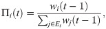
From the generated temporal networks, we first measure the degree and weight distributions of the time-aggregated networks, as shown in Fig 8(A). For all cases, P(k)s are binomial distributions as expected from the assumption that a_i = a for all nodes i, and P(w)s show heavy tails due to the preferential activation mechanism. Then, by applying the MSE method to the time series of {K(t)} and {W(t)}, we calculate $$ \overline{S_E^K}$$ and $$ \overline{S_E^W}$$ with their standard deviations, as shown in Fig 8(B)–8(D). It turns out that our temporal network model successfully generates various temporal interaction patterns observed in the empirical datasets using the above parameter values of (t_h, λ_K,h/λ_K,l, λ_L,h/λ_L,l). For example, in Fig 8(D), $$ \overline{S_E^K}$$ ($$ \overline{S_E^W}$$) shows overall increasing (flat) behaviors, which have been observed in the analysis of datasets for school (2011), school (2012), and conference [see Fig 4(D)–4(F)].

Fig 8

Simulation results of the temporal network model.

(A) Degree and weight distributions of time-aggregated networks and (B–D) the results by the MSE method applied to {K(t)} (top panels) and {W(t)} (bottom panels), denoted as $$ \overline{S_E^K}$$ and $$ \overline{S_E^W}$$, respectively. For each combination of parameter values (t_h, λ_K,h/λ_K,l, λ_L,h/λ_L,l) = (200, 3, 1) (“Case 1”), (100, 3, 1) (“Case 2”), and (100, 9, 1.5) (“Case 3”), we generate 10³ temporal networks using the fixed values of N = 100, K = 1000, W = 10000, T = 2000, ρ_K = 0.2, ρ_L = 0.8, and n = 5. In panel (A), degree distributions P(k) are linearly binned, while weight distributions P(w) are logarithmically binned.

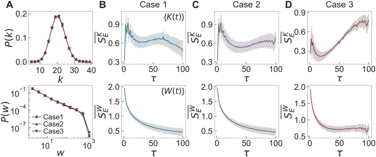
Although we do not observe broad degree distributions in the empirical datasets analyzed, we test the effect of heterogeneous activities on the network structure. In many real-world networks, the activities of nodes are known to be heterogeneous [1, 2, 4, 6–9]. We generate temporal networks using F(a) ∼ a^−γ with γ = 2.5 for networks of size N = 10⁴, whereas other parameters have the same values as in Fig 8. In Fig 9(A), we find that P(k)s of the time-aggregated networks in all cases are essentially the same, also showing heavier tails than F(a). For comparison, we calculate the P(k) in the case when every node has the chance to get activated at each time step as in the original model [24]: As expected, we find the same power-law exponent in P(k) as γ in F(a) [see the “Null” case in Fig 9(A)]. Thus, heavier tails of P(k)s in our model might be due to the limited activations of nodes by K(t), effectively enhancing the activations of more active nodes than less active ones.

Fig 9

Simulation results of the temporal network model considering heterogeneous activities of nodes or the community property.

(A) The networks are generated with F(a) ∼ a^−2.5 and N = 10⁴, and the other parameters are the same as in Fig 8. (B) and (C) The networks are generated with N_c = 5 in the same parameter settings as in Fig 8. In the panels (A) and (B), degree distributions P(k)s are logarithmically and linearly binned, respectively. In the panel (C), the modularity Q is shown for various p. Each empty marker presents the empirical result for the primary school (✰), hospital (△), workplace (▽), school (2011) (○), and school (2012) (□).

In addition, we also study the effect of community structure, such as classes in school, by considering N_c non-overlapping communities with N/N_c nodes in each community. Each of K(t) activated nodes at the time step t may create a link to another random node that belongs to the same community or another community. We define a parameter p as the ratio of the probability that the activated node chooses a neighbor node from one of other communities to the probability that the activated node chooses a neighbor node belonging to the same community. If p = 0, no links between nodes in different communities are created, while when p = 1, the activated node randomly chooses its neighbor node from the entire network, leading to the network without community structure.

We generate temporal networks for N_c = 5 with the same parameter values as in Fig 8, also assuming that a_i = a for all nodes i. Fig 9(B) and 9(C) respectively show the degree distribution P(k) and modularity Q [78] of the time-aggregated networks for various p. When p = 1, we obtain Q ≈ 0, which corresponds to the results in Fig 8. As p decreases, the activated nodes tend to form links with nodes belonging to the same community. As a result, Q increases, while the variance of P(k) decreases. The results show that even if the external factors have the same effect on the number of activated links, the topological structure of the network can be different depending on the connectivity patterns of nodes.

The empirical datasets we analyze provide information on the communities to which the nodes belong, except for the conference one: 11 communities in the primary school, 4 communities in the hospital, 5 communities in the workplace, 4 communities in the school (2011), and 5 communities in the school (2012). We estimate the value of p by counting the number of links within the same communities. In Fig 9(C), we plot Q of the empirical datasets as a function of p, which is presented by empty markers with the corresponding standard deviations. Each marker denotes an averaged value for the daily datasets. We can confirm that the hospital and workplace datasets have network structures with a significant difference in terms of Q, although they show similar MSE results, as shown in Fig 4(B) and 9(C). This emphasizes the observation that even if the environmental impacts on networks are similar, the topological properties can vary depending on the connectivity patterns.

By the numerical simulation of our temporal network model, we have shown how the periodic external factor, when combined with the internal factor and the preferential activation mechanism, can induce complex temporal correlations in the network-level interaction patterns over a wide range of timescales.

Finally, we remark that in our model the links are created (or activated for the first time) in different times, which may introduce some aging effects to the dynamics of temporal networks, e.g., as discussed in Ref. [28]. The different creation times of links can also affect the dynamical processes taking place in temporal networks such as spreading [79, 80]. In this sense our results highlight the need to study the impact of the environmental changes on the dynamics of temporal networks.