Statistical model

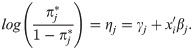
The proportional odds ordinal logistic model is an extension of the logistic model for binary outcomes and is described in full detail elsewhere [38–40]. The outcome variable Y_i of subject i = 1,…,N is ordinal with categories c₁,…,c_J and related probabilities π_j = p(Y_i = j) with $$ {\sum }_j^J{\pi }_j=1$$. The J−1 non-redundant cumulative probabilities $$ {\pi }_1^{*},\dots ,{\pi }_{j-1}^{*}$$ are defined as $$ {\pi }_j^{*}=p(Y_i\le j)$$ and for each of these a logistic regression model is formulated

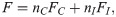
The model parameters θ′ = (γ₁, γ₂,…,γ_J−1, β) can be estimated by means of maximum likelihood estimation, for further details see Glonek and McCullogh [42]. The associated covariance matrix $$ cov\left(\widehat{\theta }\right)$$ plays an important role in the derivation of the optimal design. An asymptotic approximation is calculated from the inverse of the Fisher information matrix F, with

Derivation of the optimal treatment allocation

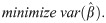
Optimal design methodology is used to derive the optimal allocation to treatments [43–45]. In this contribution the optimal allocation is sought under the condition

A special case of the constraint is when c_C = c_I = 1 and B is replaced by N. In that case the optimal design is sought under a fixed total sample size N: n_C+n_I = N. This constraint is relevant when treatments for a rare disease are compared and only a limited number of subjects can be enrolled in the trial.

The optimal design p*∈(0,1) is the optimal proportion of subjects in the intervention condition. It is found numerically as follows: for any proportion p in the interval (0,1) the sample sizes n_C and n_I are calculated from the budgetary constraint. Note that these sample sizes are not necessarily integers. These sample sizes are plugged in the Fisher information matrix F from equation (2) and the value of the optimality criterion is calculated. The optimal design is the one with the smallest value on the optimality criterion. It can be shown not to depend on the budget B or total sample size N. In the remainder of this paper a step size of 0.01 for the proportion is used to find the optimal design. As the optimal design is expressed in terms of a proportion, the optimal design is a so-called continuous or approximate optimal design. For implementation, the optimal design has to be expressed in terms of the sample sizes in both conditions, a so-called discrete or exact optimal design. Exact designs are often difficult to find. In practice, the exact optimal design is approximated by calculating n_I = p*N and rounding to the nearest integer value and calculating n_C = N−n_I.

Note that it is also possible to minimize the budget (or total sample size) so that a certain value for the variance of the treatment effect estimator, and hence a certain power for the test on treatment effect, is achieved. This will result in the same optimal proportion p* as when the variance is minimized given a fixed budget B (or total sample size N).

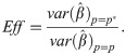
The performance of all other designs p as compared to the optimal design p* can be expressed in terms of their efficiencies. The efficiency of a design is calculated as

A Shiny App is available to help the reader find the optimal allocation for a specific study at hand and to evaluate the efficiency of other designs, including the balanced design. It considers three to seven ordered response categories (https://utrecht-university.shinyapps.io/OD_Ordinal/). The Shiny App also shows the relation between the power for the test on treatment effect and the budget, for both the optimal design and the balanced design. This graph shows what power level can be obtained for a given budget, or how large the budget should be to achieve a certain desired power level. To derive the optimal design a prior estimate of the treatment effect size must be given. The robustness graph shows how well the optimal design performs if this prior estimate is different from the population value. The code for this Shiny App is available at https://github.com/MirjamMoerbeek/OD_Ordinal.

Optimal treatment allocations

This subsection shows how the number of response categories, the response probabilities in these categories, the treatment effect size and constraint influence the optimal allocation. Results are presented for three, five or seven categories. The response probabilities in the control condition are the same as those in Bauer and Sterba [46] and are depicted in Fig 1. Three distributions are taken into account: bell-shaped, skewed and polarized. The probabilities in the intervention follow from a proportional odds model with a treatment effect size (expressed as an odds ratio: OR = e^β) of 1.68, 3.47 and 6.71, which are small, medium and large effect sizes [47]. A fixed total sample size is used (i.e. c_I/c_C = 1), as well as a budgetary constraint with cost ratios c_I/c_C = 2 and 5.

Fig 1

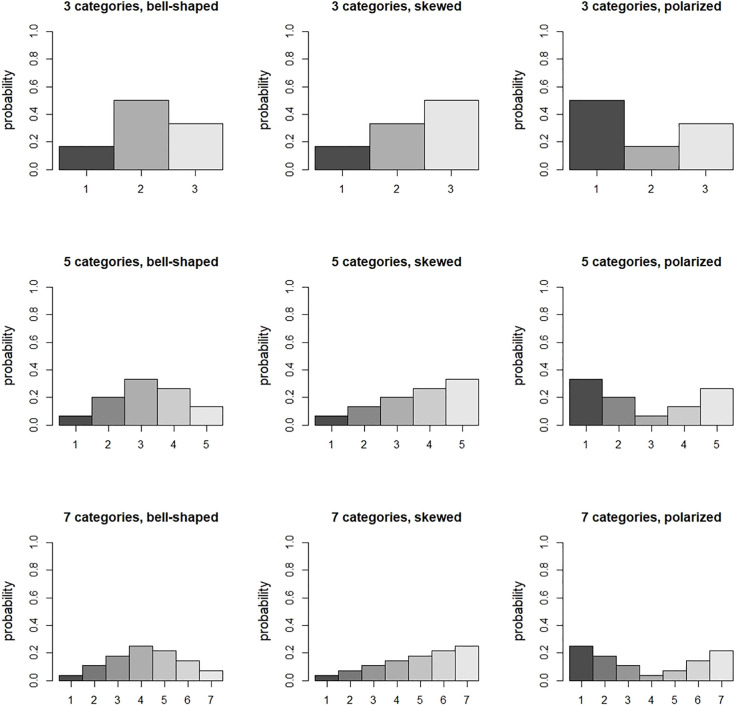
Response probabilities in the control condition.

Tables 1–3 present the optimal proportion of subjects in the intervention and the efficiency of the balanced design for three, five and seven response categories, respectively. The following findings are observed with respect to the optimal proportion:

For the polarized distribution the optimal proportion increases with increasing effect size, especially so for small number of categories. For the other two distributions the relation is either absent or slightly decreasing.

The optimal proportion decreases when the cost ratio increases. This implies the optimal proportion for a fixed total sample size (i.e. c_I/c_C = 1) is larger than for a fixed budget (i.e. c_I/c_C>1).

For the polarized distribution the optimal proportion decreases with increasing number of categories. For the other two distributions the relation is absent

The optimal proportion depends on the distribution of the response probabilities. It is highest for the polarized distribution.

Table 1

Optimal proportion of subjects in the intervention [efficiency of the balanced design] for three response categories.

cost ratio = 1a
OR	bell-shaped	skewed	polarized
1.68	0.50 [1.00]	0.49 [1.00]	0.52 [1.00]
3.47	0.50 [1.00]	0.50 [1.00]	0.56 [0.99]
6.71	0.50 [1.00]	0.50 [1.00]	0.67 [0.96]
cost ratio = 2
OR	bell-shaped	skewed	polarized
1.68	0.41 [0.97]	0.41 [0.97]	0.43 [0.98]
3.47	0.40 [0.97]	0.40 [0.97]	0.47 [1.00]
6.71	0.40 [0.96]	0.41 [0.97]	0.52 [1.00]
cost ratio = 5
OR	bell-shaped	skewed	polarized
1.68	0.31 [0.87]	0.30 [0.86]	0.32 [0.89]
3.47	0.29 [0.86]	0.29 [0.86]	0.36 [0.94]
6.71	0.28 [0.85]	0.29 [0.86]	0.41 [0.98]

^aCost ratio = 1 implies a fixed total sample size.

Table 2

Optimal proportion of subjects in the intervention [efficiency of the balanced design] for five response categories.

cost ratio = 1a
OR	bell-shaped	skewed	polarized
1.68	0.50 [1.00]	0.50 [1.00]	0.51 [1.00]
3.47	0.50 [1.00]	0.50 [1.00]	0.53 [1.00]
6.71	0.50 [1.00]	0.50 [1.00]	0.56 [0.99]
cost ratio = 2
OR	bell-shaped	skewed	polarized
1.68	0.41 [0.97]	0.41 [0.97]	0.42 [0.97]
3.47	0.41 [0.97]	0.41 [0.97]	0.44 [0.99]
6.71	0.40 [0.97]	0.40 [0.97]	0.47 [1.00]
cost ratio = 5
OR	bell-shaped	skewed	polarized
1.68	0.31 [0.87]	0.30 [0.87]	0.31 [0.88]
3.47	0.30 [0.86]	0.29 [0.86]	0.33 [0.90]
6.71	0.28 [0.85]	0.28 [0.85]	0.35 [0.93]

^aCost ratio = 1 implies a fixed total sample size.

Table 3

Optimal proportion of subjects in the intervention [efficiency of the balanced design] for seven response categories.

cost ratio = 1a
OR	bell-shaped	skewed	polarized
1.68	0.50 [1.00]	0.50 [1.00]	0.50 [1.00]
3.47	0.50 [1.00]	0.50 [1.00]	0.52 [1.00]
6.71	0.50 [1.00]	0.50 [1.00]	0.54 [1.00]
cost ratio = 2
OR	bell-shaped	skewed	polarized
1.68	0.41 [0.97]	0.41 [0.97]	0.42 [0.97]
3.47	0.41 [0.97]	0.41 [0.97]	0.42 [0.98]
6.71	0.40 [0.97]	0.40 [0.97]	0.44 [0.99]
cost ratio = 5
OR	bell-shaped	skewed	polarized
1.68	0.31 [0.87]	0.31 [0.87]	0.31 [0.88]
3.47	0.29 [0.86]	0.29 [0.86]	0.31 [0.88]
6.71	0.28 [0.85]	0.28 [0.85]	0.33 [0.91]

^aCost ratio = 1 implies a fixed total sample size.

For a fixed total sample size the optimal proportion for the bell-shaped and skewed distribution is most often near 0.5 and the efficiency of the balanced design is higher than 0.95. For cost ratios c_I/c_C = 2 and 5 the optimal proportion of subjects in the intervention is almost always less than 0.5. The further the optimal proportion is away from 0.5, the lower the efficiency of the balanced design. This efficiency is always larger than 0.8 for the chosen cost ratios. However, for larger cost ratios the efficiency further decreases. For instance, c_I/c_C = 20 it is equal to 0.71 for a bell-shaped distribution with three categories and a small effect size. It can thus be concluded that the balanced design is not always the best choice.

Robustness of the locally optimal designs

For any combination of the number of response categories and cost ratio, the optimal proportions in Tables 1–3 are locally optimal, meaning that they depend on the parameters of the ordinal logistic model: the thresholds (i.e. distribution of response probabilities) and treatment effect size [48]. For any cost ratio and number of categories, the optimal proportions for the bell-shaped and skewed distributions are rather similar and they show a weak or absent relation with the effect size. The optimal proportions for the polarized distribution are most often different from those of the other two distributions and are stronger related with the effect size.

To calculate the optimal design one must specify the response probabilities in each of the categories, along with the treatment effect size. Prior estimates can be obtained from an expert’s knowledge or expectations, the literature or a pilot study. However, there is always a risk these prior estimates are incorrect, meaning they are different from the population values. It is therefore important to assess the robustness of the locally optimal design against a misspecification of the prior estimates of the model parameters. For each combination of distribution of response probabilities and treatment effect size the efficiency of the optimal design was calculated for any other such combination. In other words, it was studied how well the optimal design for an incorrect prior estimate of these model parameters performs under the true population values of model parameters. Almost all optimal designs in Tables 1–3 have an efficiency of at least 0.9 for the other eight combinations of distribution of response probabilities and effect size. Only one of them has an efficiency that is lower than 0.9, but still above 0.85. It is the optimal design sought under a fixed total sample size, for the polarized distribution with three categories and OR = 6.71. The efficiency of this design is 0.88 or 0.89 in the case the distribution is bell-shaped or skewed with OR = 1.68 or OR = 3.47. In general it can be concluded that the locally optimal designs are highly robust with respect to misspecification of the model parameters.

For any study, the robustness graph in the Shiny app can be used to evaluate the robustness of an optimal design based on a prior estimate of the effect size if the population value is different from this prior estimate.

Example 1: Treatment for schizophrenia

The psychiatric example in section 10.3 of Hedeker and Gibbons [33] uses data from the National Institute of Mental Health Schizophrenia Collaborative Study. In this trial 108 schizophrenic patients were randomized to placebo and 329 to anti-psychotic drug. The drug group consisted of three different drugs, but since previous analyses revealed similar effects these drug groups were combined. The outcome ‘severity of illness’ was categorized into four ordered categories: normal, mildly or moderately ill, markedly ill, and severely ill. At baseline there were no differences between the two treatment groups with respect to the outcome ($$ \widehat{\beta }=-0.09,p=0.406,OR=0.92$$). Three weeks after baseline the outcome was observed on 87 patients in the placebo condition and 287 in the drug condition. A proportional odds model showed the effect of condition was significant ($$ \widehat{\beta }=1.217,p<0.001,OR=3.377$$). The estimated thresholds were $$ {(\widehat{\gamma }}_1,{\widehat{\gamma }}_2,{\widehat{\gamma }}_3)=(-2.79,-\mathrm{0.96,0.52})$$, which corresponds to probabilities in the control (p₁, p₂, p₃, p₄) = (0.06,0.22,0.35,0.37). The estimated probabilities in both conditions are shown in Fig 2; better results are observed in the drug group. The Brant test shows the proportional odds assumption is not violated (χ² = 3.13, df = 2, p = 0.21).

Fig 2

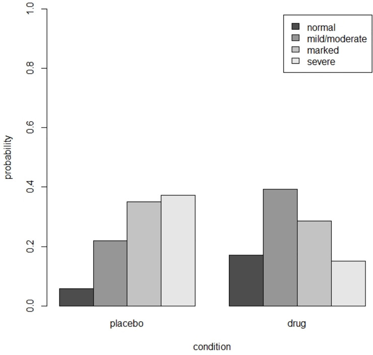
Estimated probabilities in the placebo and drug condition for the schizophrenia example.

Suppose this trial is to be replicated such that the power for any given sample size is maximized. A relevant question is whether a design with an equal number of subjects per treatment condition is the most efficient. The design is locally optimal and the parameter estimates as given above are used to derive the optimal design. Fig 3 shows the efficiencies as a function of the proportion of patients in the drug condition. The optimal proportion is p* = 0.50, which implies the optimal design is the balanced design. This optimal design is highly robustness to an incorrect prior guess of the treatment effect: for any population value of the treatment effect in the range OR = [0.1,10] its efficiency is at least 0.96.

Fig 3

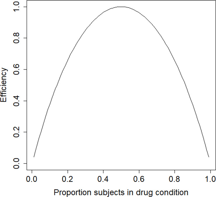
Efficiency graph for the schizophrenia example.

A relevant question is how large the sample size should be to detect at treatment effect of size β = 1.217 with a power level of 0.8 in a test with type I error rate of 0.05 and a one-sided alternative hypothesis. Fig 4 shows the relation between total sample size and power. The total sample size can be calculated to be 61, which is much lower than in the original study.

Fig 4

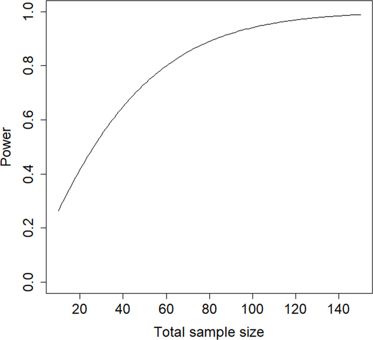
Power graph for the schizophrenia example.

Example 2: Treatment for trauma

This example uses data from Chuang-Stein and Agresti [34]. Five ordered categories describe the clinical outcome of patients who experienced trauma: death, vegetable state, major disability, minor disability and good recovery. These are often called the Glasgow Outcome Scale. There were four treatment groups based on the dose level of the investigational medication: placebo (n = 210), low dose (n = 190), medium dose (n = 207) and high dose (n = 195).

Suppose this trial has to be replicated and interest is in the comparison of placebo versus medium dose. A proportional odds model shows the estimated treatment effect is of small size and insignificant at $$ \alpha =0.05(\widehat{\beta }=-0.324,p=0.064,OR=0.723)$$. The estimated thresholds are $$ {(\widehat{\gamma }}_1,{\widehat{\gamma }}_2,{\widehat{\gamma }}_3,{\widehat{\gamma }}_4)=(-0.95,-\mathrm{0.50,0.49,1.90})$$, which corresponds to probabilities in the control (p₁, p₂, p₃, p₄, p₅) = (0.28,0.10,0.24,0.25,0.13). The estimated probabilities in both conditions are shown in Fig 5; more favorable results are observed in the drug group. The proportional odds assumption is not violated (Brant test: χ² = 4.86, df = 3, p = 0.18).

Fig 5

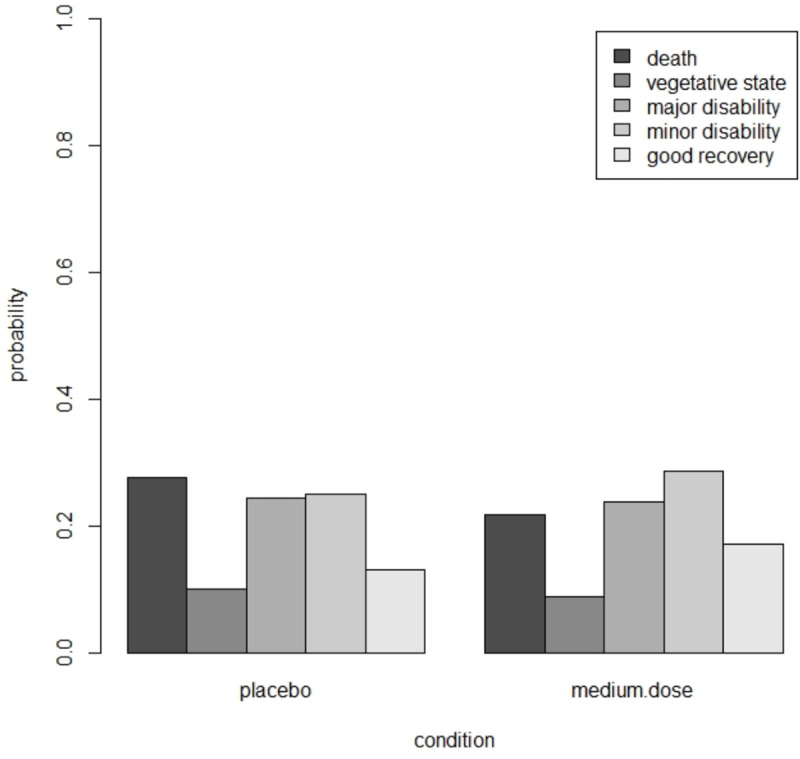
Estimated probabilities in the placebi and medium dose group in the trauma example.

In the derivation of the optimal design we assume differential costs across the two treatments, with a cost ratio c_I/c_C = 2.5. The estimated treatment effect and thresholds are used to derive the locally optimal design. Fig 6 shows the efficiency plot. The optimal proportion of subjects in the medium dose drug condition is p* = 0.39 and the efficiency of the balanced design is 0.95. The balanced design is highly efficient but not the best choice. The optimal design is highly robust to an incorrect prior estimate of the treatment effect size. For any population value of the treatment effect in the range OR = [0.1,10] it has an efficiency of at least 0.99.

Fig 6

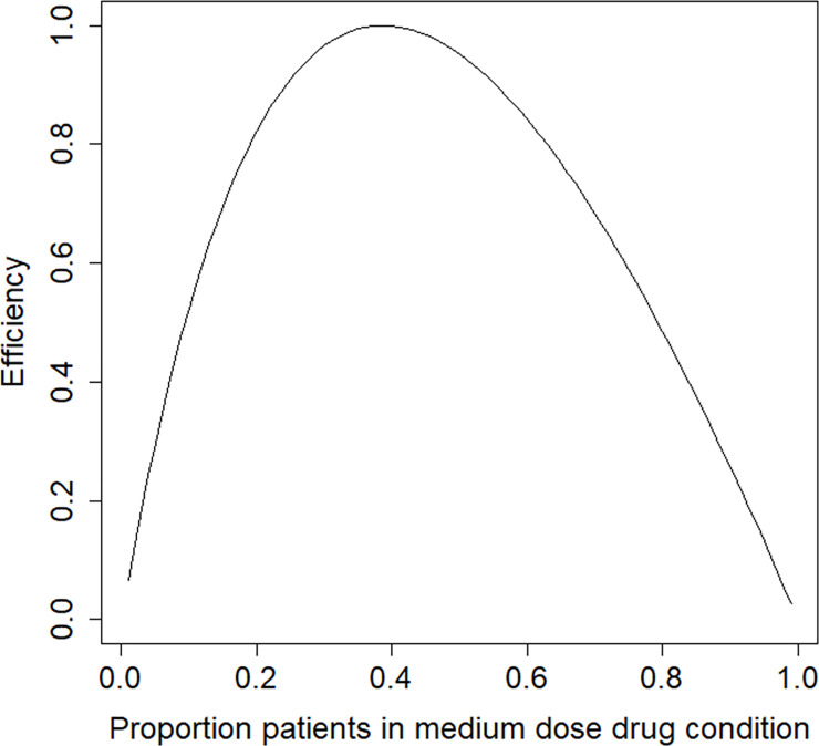
Efficiency graph for the trauma example.

Fig 7 shows the relation between budget and the power to detect a treatment effect of β = −0.324 in a one-sided test with a type I error rate of 0.05. The costs are scaled so that c₁ = 1; in other words, the budget is expressed in terms of the costs per subject in the control condition. To achieve a power of 0.8 for the test on treatment effect at a type I error rate of 0.05 and a one sided alternative a budget of B = 1262 is needed. The corresponding total sample size is 796, which is almost twice as high as in the original study.

Fig 7

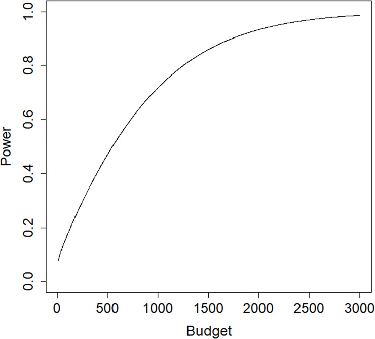
Power graph for the trauma example.