 Index tracking strategy based on mixed-frequency financial data
PLoS ONE


Competing Interests: The authors have declared that no competing interests exist.

- Altmetric
To obtain market average return, investment managers need to construct index tracking portfolio to replicate target index. Currently, most literatures use financial data that has homogenous frequency when constructing the index tracking portfolio. To make up for this limitation, we propose a methodology based on mixed-frequency financial data, called FACTOR-MIDAS-POET model. The proposed model can utilize the intraday return data, daily risk factors data and monthly or quarterly macro economy data, simultaneously. Meanwhile, the out-of-sample analysis demonstrates that our model can improve the tracking accuracy.
Introduction
The index tracking strategy, which aim at tracking the return of a given stock index when constructing the portfolio, is a major strategy adopted by fund managers. [1–7] theoretically and experimentally study the index tracking strategy under different constraints in reality, e.g. the number of stocks in the portfolio is limited.
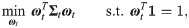
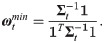
The simplest and most widely used index tracking strategy is the global minimum variance strategy. Let Rt be the vector of daily excess returns of stocks over the target index and ωt be the global minimum variance portfolio weights. The difference between return of the index tracking strategy and return of the target index is on day t. Mathematically, the investors aim to minimize tracking error, which is measured by variance of the difference between return of the index tracking strategy and return of the target index, i.e.,
In the literature, methods for estimating the covariance matrix or inverse covariance matrix mainly focus on financial data with homogenous frequency. [8–10] try to estimate the covariance matrix based on quarterly, monthly and daily returns, respectively. [5, 11–18] aim to improve covariance matrix estimation using intraday data. Differently [19–23], focus on the estimation of inverse covariance matrix. With the improvement in high-speed computation and large amounts of storage, financial data streams become more and more real-time and complex, such as high-frequency data and ultra-high-frequency data. Besides the historical data in financial markets, monthly or quarterly macro-economic factors are also valuable information sources of stocks’ volatilities (see [24–29] further reveal that macro-economic factors, such as GDP growth, exchange rate and short-term interest rate, are important explanatory variables of the slow-moving component in volatilities.
However, due to the heterogeneous frequency of macro-economic factors and historical data, it is a great challenge to construct a unified econometric model. Among all proposed models, the mixed data sampling (MIDAS) method in [30] attracts great attentions, and induces several important extensions, such as GARCH mixed-data sampling (GARCH-MIDAS) model (see [31]), Factor-based mixed-data sampling (Factor-MIDAS) model (see [32]). Different from the MIDAS method, other economic models handling mix-frequency data, such as High-frequency-based volatility (HEAVY) model (see [33]); Factor GARCH-Itô model (see [34]), are mainly focusing on integrating the intraday financial data and daily financial data. Compared with homogenous-frequency models, mixed-frequency model contains more information in the original data, which can better capture market and have better accuracy in prediction. It provides a timely update on portfolio and helps fund managers achieve targeted index tracking performance.
In this paper, we propose a general framework for mixed-frequency financial data, called FACTOR-MIDAS-POET model, to estimate the covariance matrix. The proposed model combines monthly macro-economic factors, daily observable factors (market return and the innovation of VIX) and intraday returns to improve covariance matrix estimation. In empirical analysis, we compare our model with existing models in the literature, and find that the tracking accuracy of minimum variance tracking strategy is greatly improved by using the proposed model. The reason is that compared with other models, our model contains macro-economic information and option market information. We also find that when the amount of historical data decreases, performances of the index tracking portfolios based on different models all decrease, but our model is less affected. Moreover, when the estimation window is short (e.g., 3 months), integrating intraday return data into our model may yield better tracking performance than not using the intraday return data.
The remaining paper is organized as follows. In the estimations of the covariance and its inverse, we introduce existing methods for estimating the covariance matrix and inverse covariance matrix based on homogenous frequency data. In FACTOR-MIDAS-POET method and estimation, we introduce the FACTOR-MIDAS-POET model and its estimation method. In data and descriptive analysis, we explain the data used in this paper. In empirical study, we conduct the empirical study and compare performances of different models. In conclusions and discussion, we conclude our paper.
The estimations of the covariance and its inverse
To obtain the minimum variance index tracking strategy, there are two main ways. The first one is to estimate the covariance matrix and then obtain the inverse matrix; The second one is to estimate the inverse covariance matrix directly. The rest of this section summarizes the important existing methods for estimating the covariance matrix and inverse covariance matrix.
Estimators of covariance matrix
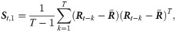
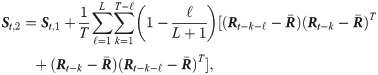
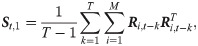
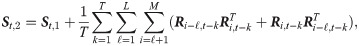
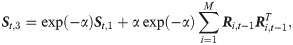
Based on the daily financial data, we summarize three estimators as follows,

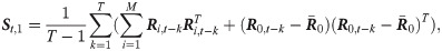
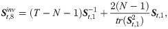
When we have intraday financial data, these estimators are modified as follows,

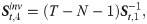
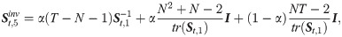
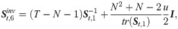
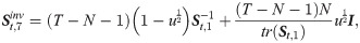
Estimators of inverse covariance matrix
The estimators of inverse covariance matrix are often built upon the estimators of covariance matrix. We summarize these estimators in this subsection.
FACTOR-MIDAS-POET method and estimation
There are two restrictions of the methods summarized in Section 2. The first one is that these classical methods require a homogenous sampling frequency, leading to a low usage of information contained in mixed-frequency financial data; The second is that these classical methods do not take monthly or quarterly macro-economic factors into consideration. To remedy these limitations, we propose a model involving multi-frequency financial data to better reflect financial market.
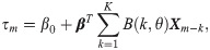
In our model, excess returns are driven by both observable and unobservable factors. Meanwhile, excess returns are influenced by the status of macro economy. More specifically, the model is shown as follows,

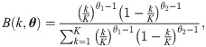
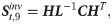
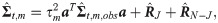
Based on principal orthogonal complement thresholding(POET) method in [37], the daily covariance matrix of excess returns, , is estimated as follows,
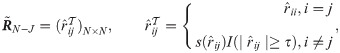

Based on [38], we apply the method of linear compression to obtain the shrinkage inverse covariance matrix estimator as follows:
Data and descriptive analysis
Data
In empirical analysis, we use the stocks listed in Dow Jones Industrial Average (DJIA) to track the S&P 500 index. The stock tickers and full company names of 30 stocks listed in DJIA are available in Table 1. As there are too many missing values in the TAQ data files of TRV company, we remove this company and use the rest 29 DJIA stocks to track S&P 500 index. The sample period in our analysis is from Jan. 1st, 2006 to Dec. 31st, 2011. The daily and 5 minutes (5-min) data of S&P 500 index are obtained from Tick Data. The 5-min data of 30 DJIA stocks are collected from NYSE Trade and Quotations (TAQ) database. Considering the higher possibility of including biases and reporting errors in the first 30 minutes after opening, we discard the first 30 minutes data. Thus, there are 72 intraday 5-min returns and one overnight return in each trading day.

| Ticker | Company Name |
|---|---|
| AA | Alcoa Inc. |
| AXP | American Express Company |
| BA | The Boeing Company |
| BAC | Bank of America Corporation |
| CAT | Caterpillar Inc. |
| CSCO | Cisco Systems, Inc. |
| CVX | Chevron Corporation |
| DD | E.I. du Pont de Nemours & Company |
| DIS | The Walt Disney Company |
| GE | General Electric Company |
| HD | The Home Depot, Inc. |
| HPQ | Hewlett-Packard Company |
| IBM | International Business Machines Corporation |
| INTC | Intel Corporation |
| JNJ | Johnson & Johnson |
| JPM | JPMorgan Chase & Co. |
| KFT | Kraft Foods Inc. |
| KO | The Coca-Cola Company |
| MCD | McDonald’s Corporation |
| MMM | 3M Company |
| MRK | Merck & Co., Inc. |
| MSFT | Microsoft Corporation |
| PFE | Pfizer Inc. |
| PG | The Procter & Gamble Company |
| T | AT&T Inc. |
| TRV | The Travelers Companies, Inc. |
| UTX | United Technologies Corporation |
| VZ | Verizon Communications Inc. |
| WMT | Wal-Mart Stores, Inc. |
| XOM | Exxon Mobil Corporation |
The daily value-weighted market return and daily VIX are considered as daily observable factors and obtained from CRSP database and Chicago Board Options Exchange (CBOE), respectively.
The monthly macro-economic factors includes eight important ones:
Short-term interest rate (Interest), which is measured by 3-month US treasury bill rate and obtained from the Federal Reserve Board’s H.10.
Exchange rate (Exch.), which is measured by the major currencies index collected from Federal Reserve Banks and obtained from the Federal Reserve Board’s H.15.
Inflation (Inflation), which is measured by the Consumer Price Index (CPI) and obtained from CRSP database.
Slope of the yield curve (Slope), which is measured by the spread between 10-year treasury rate and 3-month treasury rate and obtained from CRSP database.
Default rate (Default), which is measured by the difference between Moody’s Baa and Aaa corporate bond yields of the same maturity and obtained from Federal Reserve Board data files in WRDS database.
Consumer confidence (CC), which is measured by the Michigan Consumer Sentiment Index and obtained from Trading Economics.
Growth rate in the Industrial Production Index (IPI), which is obtained from Federal Reserve Board data files in WRDS database.
Unemployment rate (Unempl.), which is obtained from Trading Economics.
Utilizing the method in [28], we conduct the Principle Components Analysis (PCA) to these eight variables and select the first two principle components as macro-economic factors used in our model.
Descriptive analysis
Tables 2 and 3 present the descriptive statistics for daily returns and 5-min returns of 29 DJIA stocks and S&P index, respectively.
| Stock | Mean × 1000 | 25th Percentile × 1000 | 75th Percentile × 1000 | SD × 1000 | Skewness | Kurtosis |
|---|---|---|---|---|---|---|
| AA | -0.8021 | -14.7440 | 15.0712 | 33.2524 | -0.2453 | 5.8662 |
| AXP | -0.0798 | -11.0745 | 11.5691 | 29.8404 | 0.1049 | 6.4575 |
| BA | 0.0286 | -10.2271 | 10.7482 | 20.7952 | 0.1065 | 3.6824 |
| BAC | -1.3867 | -13.5525 | 10.9586 | 43.5349 | -0.2921 | 13.7690 |
| CAT | 0.3155 | -11.6219 | 12.8381 | 24.0225 | -0.0728 | 3.5591 |
| CSCO | 0.0425 | -9.8890 | 10.7245 | 21.5366 | -0.2270 | 6.6922 |
| CVX | 0.4070 | -8.9778 | 10.5710 | 19.6762 | 0.1361 | 11.2978 |
| DD | 0.0494 | -10.1948 | 10.6622 | 20.7331 | -0.4140 | 4.6500 |
| DIS | 0.3111 | -9.2823 | 9.6864 | 19.9378 | 0.3029 | 5.8237 |
| GE | -0.4444 | -8.9738 | 8.8330 | 23.1800 | -0.1263 | 6.7691 |
| HD | 0.0271 | -10.1650 | 10.0027 | 20.0926 | 0.3543 | 3.3508 |
| HPQ | 0.0150 | -9.4746 | 10.4959 | 20.4492 | 0.0518 | 4.1362 |
| IBM | 0.5299 | -6.5984 | 8.3069 | 15.1777 | 0.0212 | 4.2217 |
| INTC | -0.0186 | -10.7499 | 11.1148 | 21.0361 | -0.1867 | 3.7357 |
| JNJ | 0.0490 | -4.7435 | 5.2749 | 10.9609 | 0.1181 | 10.1205 |
| JPM | -0.1124 | -12.3190 | 11.2466 | 32.5366 | 0.3622 | 9.9782 |
| KFT | 0.1963 | -6.4856 | 7.1668 | 13.5095 | 0.0097 | 3.8798 |
| KO | 0.3546 | -5.5730 | 6.0818 | 12.7197 | 0.4636 | 8.5198 |
| MCD | 0.7355 | -6.5178 | 7.8164 | 13.4517 | -0.0439 | 3.8460 |
| MMM | 0.0280 | -6.8518 | 8.0256 | 16.3772 | -0.3299 | 4.7732 |
| MRK | 0.1455 | -8.4768 | 9.4536 | 18.6671 | -0.2957 | 6.2243 |
| MSFT | -0.0063 | -8.6208 | 8.7621 | 18.9069 | 0.1018 | 8.1691 |
| PFE | -0.0239 | -7.9898 | 8.3449 | 16.1736 | -0.0495 | 4.5433 |
| PG | 0.0897 | -4.8103 | 5.5626 | 12.1929 | -0.1406 | 7.2973 |
| T | 0.1492 | -7.7032 | 7.9086 | 16.2232 | 0.5071 | 8.2793 |
| UTX | 0.1827 | -7.6566 | 8.8274 | 17.4147 | 0.2696 | 5.8673 |
| VZ | 0.1781 | -7.0986 | 8.0542 | 15.8020 | 0.2347 | 7.0804 |
| WMT | 0.2052 | -6.7874 | 6.5878 | 13.1521 | 0.1291 | 5.5092 |
| XOM | 0.2658 | -8.1494 | 9.2605 | 18.2490 | -0.0163 | 13.0925 |
| S&P 500 | 0.0485 | -5.4778 | 6.4014 | 15.3059 | -0.1909 | 7.4016 |
| Stock | Mean × 1000 | 25th Percentile × 1000 | 75th Percentile × 1000 | SD × 1000 | Skewness | Kurtosis |
|---|---|---|---|---|---|---|
| AA | -0.0170 | -1.1251 | 1.1036 | 2.6924 | -0.0922 | 15.9145 |
| AXP | 0.0135 | -0.8775 | 0.8809 | 2.5181 | 0.2917 | 22.9642 |
| BA | -0.0011 | -0.7457 | 0.7478 | 1.7395 | -0.2040 | 21.3570 |
| BAC | -0.0240 | -0.9307 | 0.8824 | 3.2044 | -0.1366 | 32.5194 |
| CAT | 0.0009 | -0.9121 | 0.9187 | 2.1086 | 0.2842 | 12.7307 |
| CSCO | -0.0089 | -0.8504 | 0.8252 | 1.8720 | 0.1516 | 15.1925 |
| CVX | 0.0011 | -0.7753 | 0.7882 | 1.7979 | -0.0055 | 20.2444 |
| DD | -0.0002 | -0.8005 | 0.8066 | 1.8509 | -0.2325 | 25.5643 |
| DIS | 0.0083 | -0.7163 | 0.7307 | 1.7045 | -0.0389 | 23.6222 |
| GE | -0.0041 | -0.7620 | 0.7504 | 2.1056 | 0.4918 | 28.2999 |
| HD | 0.0017 | -0.8085 | 0.7973 | 1.8943 | 0.1044 | 13.9980 |
| HPQ | 0.0027 | -0.7484 | 0.7581 | 1.7736 | 1.1672 | 82.0893 |
| IBM | 0.0048 | -0.5913 | 0.6060 | 1.4757 | -0.6339 | 44.7640 |
| INTC | -0.0037 | -0.8559 | 0.8544 | 1.8677 | -0.0364 | 24.9960 |
| JNJ | 0.0022 | -0.4437 | 0.4413 | 1.0765 | -0.4679 | 49.5585 |
| JPM | 0.0002 | -0.9356 | 0.9266 | 2.6568 | 0.0829 | 23.6656 |
| KFT | 0.0061 | -0.5369 | 0.5497 | 1.2937 | 0.0724 | 22.4096 |
| KO | 0.0020 | -0.4996 | 0.5029 | 1.1862 | -0.0108 | 22.3711 |
| MCD | 0.0034 | -0.5607 | 0.5792 | 1.3207 | -0.1335 | 21.7493 |
| MMM | 0.0015 | -0.6413 | 0.6412 | 1.4869 | -0.0982 | 22.6983 |
| MRK | -0.0012 | -0.7006 | 0.7023 | 1.6773 | 0.1270 | 49.9546 |
| MSFT | -0.0036 | -0.7170 | 0.7134 | 1.6315 | -0.0946 | 13.9688 |
| PFE | -0.0052 | -0.6988 | 0.6874 | 1.5323 | -0.0156 | 16.3319 |
| PG | 0.0008 | -0.5052 | 0.5132 | 1.2062 | -0.5129 | 50.5912 |
| T | -0.0004 | -0.6514 | 0.6497 | 1.6550 | -0.4433 | 32.2104 |
| UTX | 0.0046 | -0.6504 | 0.6588 | 1.5672 | -0.2740 | 37.8865 |
| VZ | 0.0064 | -0.6205 | 0.6364 | 1.5476 | 0.0266 | 27.5602 |
| WMT | -0.0010 | -0.5837 | 0.5779 | 1.3347 | 0.5412 | 30.5054 |
| XOM | 0.0003 | -0.7262 | 0.7444 | 1.6712 | -0.1574 | 25.4161 |
| S&P 500 | 0.0009 | -0.5111 | 0.5183 | 1.3497 | 0.0440 | 22.5620 |
Although the mean of daily returns and 5-min returns for S&P 500 index are approximately zero, their standard deviations are significantly different. It indicates that when sampling frequency increase, there is a dramatic change in volatility. Moreover, the skewness switches from -0.1909 for daily return to 0.0440 for 5-min return, which is more right-skewed. The kurtosis increases from 7.4016 for daily return to 22.5620 for 5-min return.
The standard deviations of individual stocks obtained from daily returns are significantly larger than those obtained from 5-min returns. Among the 29 individual stocks, 13 stocks have left-skewed distributions for daily return and 18 stocks have left-skewed distributions for 5-min return. Furthermore, the 29 stocks have larger kurtosis for 5-min return. The distributions of individual stock return are unsymmetrical with the long tail and sharp peak.
Table 4 further displays the correlation coefficients of eight macro-economic factors. It reveals the strong correlations between short-term interest rate and slope of the yield curve, between exchange rate and default rate, between growth rate in the Industrial Production Index and unemployment rate. Introducing all macroeconomic variables in covariance estimation model at one time will lead to a lack of statistical significance due to the presence of multicollinearity. Thus, we use principal component analysis (PCA) to create new independent variables and estimate inverse covariance matrix based on principle components in empirical study.
| Interest | Exch. | Inflation | Slope | Default | CC | IPI | Unempl. | |
| Interest | 1 | |||||||
| Exch. | 0.056 | 1 | ||||||
| Inflation | 0.397 | -0.309 | 1 | |||||
| Slope | -0.521 | -0.039 | -0.333 | 1 | ||||
| Default | -0.316 | 0.512 | -0.371 | 0.163 | 1 | |||
| CC | -0.074 | -0.077 | -0.092 | -0.040 | -0.171 | 1 | ||
| IPI | 0.175 | -0.046 | 0.182 | -0.059 | -0.025 | -0.317 | 1 | |
| Unempl. | -0.053 | 0.157 | -0.142 | 0.003 | 0.087 | -0.010 | -0.417 | 1 |
Table 5 shows the principle component matrix using PCA. The first principal component and second principal component we use explain 96.4945% of the total variance. The first component has significantly correlations with short-term interest rate and slope of the yield curve, which is called monetary factor. It is viewed as an indicator of monetary policy and bond market. The second component named as economic factor has positive correlations with default rate and exchange rate, which mostly captures the periodic fluctuations in economic activity.
| Macro-economic variables | Principle component 1 | Principle component 2 |
|---|---|---|
| IPI | 0.0016 | 0.0007 |
| Default | -0.0361 | 0.1003 |
| Exch. | 0.0006 | 0.0078 |
| Inflation | 0.0019 | -0.0011 |
| Interest | 0.4148 | 0.0085 |
| Slope | -0.0257 | -0.0002 |
| Unempl. | -0.0016 | 0.0024 |
| CC | -0.0046 | -0.0212 |
Empirical study
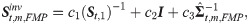
In our model, excess returns, which could be daily returns or 5-min returns, are driven by two daily observable factors: (i) the value-weighted stock market index; (ii) the innovation of the VIX index. The VIX index is constructed by the implied volatilities of S&P 500 index options. It indicates the investors’ expectation for future 30-day volatility of S&P500 index. We also include two monthly observable principle components of the eight macro-economic factors. We fit the proposed model, estimate the inverse covariance matrix, , and compute the minimum variance index tracking strategy with a rolling window scheme. And then we apply the derived strategy for the next day.
Comparison of current different estimations
Here, we choose a rolling window of one year (252 trading days). Table 6 compares out-of-sample performances of minimum variance index tracking strategies, which are derived according to different covariance matrix or inverse covariance matrix estimators based on daily return, intraday return with overnight return and intraday return without overnight return, respectivley.
| Panel A: daily return | |||||
| Covariance | SD × 100 | One-tail t test | Turnover (%) | 25th Turnover (%) | 75th Turnover (%) |
| St,1 | 4.3973 | -0.7453 | 3.3174 | 1.6897 | 4.2155 |
| St,2 | 4.9495 | -3.2205 | 6.6824 | 3.7051 | 8.2612 |
| St,3 | 4.3569 | 0.5755 | 1.5611 | 0.7266 | 1.9814 |
| 4.3973 | -0.7453 | 3.3174 | 1.6897 | 4.2155 | |
| 4.2786 | 0.9673 | 2.5055 | 1.2826 | 3.1920 | |
| 4.3805 | -0.5302 | 3.2310 | 1.6396 | 4.1386 | |
| 4.3837 | 0.1312 | 1.4594 | 0.7839 | 1.7540 | |
| 4.3943 | -0.6026 | 3.3065 | 1.6867 | 4.2125 | |
| 4.3483 | -0.4707 | 3.4507 | 1.8897 | 4.3523 | |
| Panel B: intraday return (with overnight) | |||||
| Covariance | SD × 100 | One-tail t test | Turnover(%) | 25th Turnover (%) | 75th Turnover (%) |
| St,1 | 4.5334 | -1.4928 | 1.9859 | 1.1308 | 2.2552 |
| St,2 | 4.4037 | 1.5562 | 2.1551 | 1.2385 | 2.4591 |
| St,3 | 4.5944 | -2.5103 | 1.1331 | 0.6547 | 1.2697 |
| 4.5334 | -1.4928 | 1.9859 | 1.1308 | 2.2552 | |
| 4.4053 | 0.6865 | 1.1572 | 0.7627 | 1.3270 | |
| 4.4553 | -0.7483 | 1.7850 | 1.0500 | 2.0424 | |
| 4.5583 | 1.0620 | 0.9477 | 0.6554 | 1.0710 | |
| 4.4782 | -0.6905 | 1.8969 | 1.0914 | 2.1464 | |
| 4.5042 | -2.0110 | 1.9724 | 1.1696 | 2.3179 | |
| Panel C: intraday return (without overnight) | |||||
| Covariance | SD × 100 | One-tail t test | Turnover(%) | 25th Turnover (%) | 75th Turnover (%) |
| St,1 | 4.7817 | -3.8486 | 1.8787 | 1.1561 | 2.0094 |
| St,2 | 4.4680 | 0.1306 | 2.2587 | 1.3622 | 2.4046 |
| St,3 | 4.7988 | -3.1698 | 1.1020 | 0.6804 | 1.2085 |
| 4.7817 | -3.8486 | 1.8787 | 1.1561 | 2.0094 | |
| 4.4603 | 0.3487 | 1.0710 | 0.7222 | 1.1658 | |
| 4.6069 | -2.9174 | 1.6364 | 1.0127 | 1.7634 | |
| 4.5661 | 0.4126 | 0.9483 | 0.6399 | 1.0783 | |
| 4.6563 | -3.3159 | 1.7443 | 1.0761 | 1.8579 | |
| 4.7317 | -4.1228 | 1.8818 | 1.1474 | 2.1217 | |
Notes: standard deviations are annualized.
Several conclusions can be obtained from Table 6. First, tracking error achieved by St,1 with daily return is 0.043973, which is smaller than the tracking errors of using intraday return. Second, the shrinkage inverse covariance matrix estimator, , has the best out-of-sample performance (i.e., smallest tracking error). Third, when including intraday returns, introducing overnight returns often yields better tracking performance, which implies that the overnight returns are useful. Fourth, compared with covariance matrix estimators, most inverse covariance matrix estimators do not have significantly better performances. Furthermore, Table 6 provides turnover rates of applying different strategies. The turnover rates of strategies based on intraday return are smaller, which indicates the value of intraday returns. The tracking strategy with the estimator has the lowest turnover rate.
Surprisingly, involving intraday returns may lower the tracking performance but improve the turnover rates for these estimators. What’s more, overnight returns are meaningful to improve the tracking performance.
Performance of FACTOR-MIDAS-POET method
We consider two models. The first one is based on daily returns of stocks, two daily observable factors, and two monthly macro-economic principle components. The second one is based on 5-min returns of stocks, two daily observable factors, and two monthly macro-economic principle components. Similar to [30], we estimate the models with slow weights (θ1 = 1 and θ2 = 4). We also try other forms of weights and obtain the similar conclusions.
Table 7 presents out-of-sample tracking performances of strategies based on FACTOR-MIDAS-POET model. The lag period column reports how many monthly macro-economic principle components are included in the models. Panel A presents the results based on daily returns, while Panel B and Panel C present the results based on 5-min returns. We report the one-tailed t test of tracking errors of different portfolios based on Newey-West standard deviations with six lags in Tables 6 and 7. Following [39], we examine the average squared excess returns over the target index of various estimates with the average squared excess returns of FACTOR-MIDAS-POET method (K = 3). To test the average of , , …, is significantly smaller than the average of , , …, , we test whether the mean of the sequence , , …, is significantly smaller than zero using a one-tailed test.
| Panel A: daily return | |||||
| Lag period (K) | SD × 100 | One-tail t test | Turnover (%) | 25th Turnover (%) | 75th Turnover (%) |
| 3 months | 4.3068 | 2.5313 | 1.3383 | 3.1822 | |
| 6 months | 4.3037 | 0.5512 | 2.5374 | 1.3373 | 3.1671 |
| 9 months | 4.3003 | 1.5556 | 2.5259 | 1.3181 | 3.1328 |
| 1 year | 4.2983 | 1.5215 | 2.5357 | 1.3237 | 3.1416 |
| Panel B: intraday return (with overnight) | |||||
| Lag period (K) | SD × 100 | One-tail t test | Turnover (%) | 25th Turnover (%) | 75th Turnover (%) |
| 3 months | 4.3492 | 7.9411 | 3.8282 | 10.6202 | |
| 6 months | 4.3732 | 0.8224 | 7.4164 | 3.2755 | 9.7167 |
| 9 months | 4.3968 | 0.8798 | 7.7529 | 2.5058 | 10.4505 |
| 1 year | 4.4043 | -0.4362 | 7.7152 | 2.6545 | 10.2169 |
| Panel C: intraday return (without overnight) | |||||
| Lag period (K) | SD × 100 | One-tail t test | Turnover (%) | 25th Turnover (%) | 75th Turnover (%) |
| 3 months | 4.3711 | 7.5717 | 2.6967 | 10.5070 | |
| 6 months | 4.3968 | 0.5092 | 7.1411 | 2.7568 | 9.6251 |
| 9 months | 4.4179 | 0.0177 | 7.8259 | 2.7595 | 10.4848 |
| 1 year | 4.4240 | -0.2833 | 7.8535 | 2.8240 | 10.5540 |
Some conclusions can be obtained from Table 7. First, the tracking performance and turnover ratio based on daily returns are both better than those based on 5-min returns. Second, the tracking performance of our model depends on how many monthly macro-economic principle components are included. Third, except St,3, and , the tracking performance and turnover ratio of proposed model are both better than other covariance estimation models based on daily returns. Meanwhile, the one-tail t value of St,3, and are not great. Similarly, compared with most models reported in Table 6, the proposed FACTOR-MIDAS-POET model has better out-of-sample tracking performance using intraday return. Because our method utilizes financial data with different resources and frequencies. However, the turnover rate of our model is high. This indicates that investment strategies constructed by our method are more active. The high turnover rate is not always a negative indicator. When trying to minimize the index tracking errors for investors, the index investment strategy constructed by our model can reach the targeted performance.
Robust analysis
In this robust analysis, we change the rolling window into three months (3 m), six months (6 m) and nine months (9 m), in order to check whether the length of rolling windows affects our main results.
Tables 8–10 summarize out-of-sample performances of strategies based on different models under three different lengths of rolling windows. When the length of estimation window decreases, tracking errors and turnover rates of all models increase. Because less information is used. Meanwhile, as the length of estimation window decreases, the value of 5-min return data becomes more and more important. Therefore, the intraday information can help us estimate covariance matrix or inverse covariance matrix and construct investment strategies when there is a lack of other information. Most importantly, the proposed FACTOR-MIDAD-POET model has better tracking performance than other models in general, especially when the rolling window is three months. Thus, when the length of estimation window is relatively short, introducing macro-economic information and option market information can greatly improve index tracking strategy.
| daily return | intraday return (with overnight) | intraday return (without overnight) | |||||||
|---|---|---|---|---|---|---|---|---|---|
| SD × 100 | One-tail t test | Turnover (%) | SD × 100 | One-tail t test | Turnover (%) | SD × 100 | One-tail t test | Turnover (%) | |
| St,1 | 4.3962 | -0.7695 | 4.3867 | 4.5215 | -2.5842 | 2.4893 | 4.8109 | -3.8418 | 2.2793 |
| St,2 | 5.0352 | -4.2256 | 9.6052 | 4.3443 | 0.8050 | 2.7081 | 4.4254 | -0.2626 | 2.8732 |
| St,3 | 4.3598 | 0.2221 | 1.5679 | 4.5997 | -3.0435 | 1.1360 | 4.7988 | -3.5596 | 1.1020 |
| 4.3962 | -0.7695 | 4.3867 | 4.5215 | -2.5842 | 2.4893 | 4.8109 | -3.8418 | 2.2793 | |
| 4.2696 | 0.9205 | 3.1846 | 4.3977 | -0.2501 | 1.2425 | 4.4610 | -0.6451 | 1.1080 | |
| 4.3725 | -0.4960 | 4.2268 | 4.4134 | -1.4729 | 2.1106 | 4.5698 | -3.4845 | 1.8424 | |
| 4.3613 | -0.1750 | 1.8272 | 4.5454 | 0.4413 | 0.9602 | 4.5559 | -0.4769 | 0.9560 | |
| 4.3921 | -0.2910 | 4.3656 | 4.4424 | -1.5873 | 2.3111 | 4.6302 | -3.6113 | 2.0235 | |
| 4.3237 | -0.3848 | 4.6659 | 4.4805 | -3.4180 | 2.4042 | 4.7448 | -4.0267 | 2.2522 | |
| FACTOR-MIDAS-POET Method | |||||||||
| K = 3 m | 4.3079 | 2.9523 | 4.3034 | 7.6426 | 4.3709 | 7.1357 | |||
| K = 6 m | 4.3172 | 1.3872 | 2.9439 | 4.2937 | -0.3152 | 9.3044 | 4.3606 | 1.2395 | 9.0471 |
| K = 9 m | 4.3202 | 1.2288 | 2.9333 | 4.2861 | 0.5328 | 10.2419 | 4.3515 | -0.3981 | 10.2960 |
| K = 1 y | 4.3181 | 0.7466 | 2.9268 | 4.2861 | 1.8189 | 10.5034 | 4.3491 | -0.3919 | 10.8934 |
| daily return | intraday return (with overnight) | intraday return (without overnight) | |||||||
|---|---|---|---|---|---|---|---|---|---|
| SD × 100 | One-tail t test | Turnover (%) | SD × 100 | One-tail t test | Turnover (%) | SD × 100 | One-tail t test | Turnover (%) | |
| St,1 | 4.5932 | -1.5837 | 7.1564 | 4.5772 | -1.3815 | 3.4341 | 4.9135 | -3.0659 | 2.9827 |
| St,2 | 5.6487 | -5.9653 | 17.1580 | 4.3574 | 0.0090 | 3.7923 | 4.5930 | -0.9154 | 4.1070 |
| St,3 | 4.3676 | 0.3467 | 1.5805 | 4.6044 | -2.5855 | 1.1412 | 4.7986 | -2.8346 | 1.1020 |
| 4.5932 | -1.5837 | 7.1564 | 4.5772 | -1.3815 | 3.4341 | 4.9135 | -3.0659 | 2.9827 | |
| 4.3597 | -0.5670 | 4.8490 | 4.4063 | 1.0346 | 1.3557 | 4.4801 | 0.8104 | 1.1356 | |
| 4.5404 | -1.7153 | 6.7657 | 4.3990 | -0.3520 | 2.6126 | 4.5555 | -1.5450 | 2.0895 | |
| 4.3750 | 1.1381 | 2.9238 | 4.5292 | 0.2777 | 0.9860 | 4.5485 | 0.0680 | 0.9668 | |
| 4.5829 | -2.1251 | 7.1017 | 4.4431 | -0.5275 | 3.0179 | 4.6282 | -2.0229 | 2.4208 | |
| 4.4795 | -0.4644 | 7.6952 | 4.5050 | -1.6695 | 3.2569 | 4.8155 | -3.2856 | 3.0981 | |
| FACTOR-MIDAS-POET Method | |||||||||
| K = 3 m | 4.3536 | 4.1701 | 4.2871 | 13.4000 | 4.3858 | 13.8514 | |||
| K = 6 m | 4.3482 | 1.3738 | 4.2596 | 4.3092 | 0.3213 | 12.9060 | 4.4069 | 0.1706 | 13.3304 |
| K = 9 m | 4.3475 | 1.5734 | 4.1916 | 4.3106 | 1.1315 | 12.5355 | 4.4064 | 0.0551 | 13.0920 |
| K = 1 y | 4.3467 | 1.6594 | 4.2397 | 4.3075 | 0.8631 | 12.2162 | 4.4041 | -0.0793 | 12.8645 |
| daily return | intraday return (with overnight) | intraday return (without overnight) | |||||||
|---|---|---|---|---|---|---|---|---|---|
| SD × 100 | One-tail t test | Turnover (%) | SD × 100 | One-tail t test | Turnover (%) | SD × 100 | One-tail t test | Turnover (%) | |
| St,2 | 7.5510 | -9.9487 | 54.5114 | 4.7384 | -0.1167 | 9.3569 | 5.1382 | 0.2119 | 10.7838 |
| St,3 | 4.3720 | 1.3574 | 1.6026 | 4.6092 | -2.6760 | 1.1474 | 4.7990 | -3.1201 | 1.1023 |
| 5.7823 | -4.8004 | 24.0316 | 4.7317 | -1.4858 | 6.9206 | 4.9736 | -3.0404 | 5.5949 | |
| 4.6812 | -1.1423 | 13.8312 | 4.4119 | 1.1202 | 1.4502 | 4.4645 | -0.1240 | 1.1311 | |
| 5.4748 | -3.7443 | 21.6904 | 4.2959 | 2.1670 | 3.4687 | 4.3263 | 1.3167 | 2.3255 | |
| 4.6957 | -0.6223 | 13.1463 | 4.3981 | 0.6004 | 1.1569 | 4.4206 | -0.7299 | 1.0495 | |
| 5.7178 | -4.4180 | 23.6444 | 4.3432 | 1.8964 | 4.7818 | 4.3408 | 0.8790 | 3.0793 | |
| 5.2228 | -3.1534 | 24.9688 | 4.5047 | -0.6196 | 6.0299 | 4.7502 | -3.4748 | 5.3643 | |
| FACTOR-MIDAS-POET Method | |||||||||
| K = 3 m | 4.5092 | 7.5565 | 4.3852 | 14.8179 | 4.4330 | 14.2007 | |||
| K = 6 m | 4.5023 | 0.0629 | 7.6250 | 4.3960 | -0.1793 | 14.8875 | 4.4467 | -0.3520 | 13.9836 |
| K = 9 m | 4.4996 | -0.3466 | 7.6462 | 4.4041 | -0.9606 | 14.6158 | 4.4541 | -0.6767 | 13.7511 |
| K = 1 y | 4.4993 | -0.7947 | 7.6341 | 4.4032 | -0.7387 | 14.0725 | 4.4540 | -0.6693 | 13.1841 |
Conclusions and discussion
In this paper, we propose the FACTOR-MIDAS-POET model, which integrates the intraday return data, daily risk factors data and monthly or quarterly macro economy data, simultaneously. In empirical analysis, we show that the FACTOR-MIDAS-POET model with macro-economic factors has better out-of-sample tracking performance than most current used models in the literature. The proposed model can fully utilize the financial data with different resources and frequencies. However, the better tracking performance often accompanies with higher turnover rates. Meanwhile, we find that our model has better performance as the length of the estimation window decreases.
Our work is a preliminarily study on the index tracking with mix-frequency data. There are still a lot of aspects we do not cover. For instance, we do not consider the noise of intraday data in the model. Also, when studying index tracking problems, the transaction cost is not explicitly appeared in the model. These problems are worth to be further explored in future studies.
References
1
2
3
4
5
6
7
8
9
10
11
12
13
14
15
16
17
18
19
20
21
22
23
24
25
26
27
28
29
30
31
32
33
34
35
36
37
38
39