2.1 Standard Pólya urn

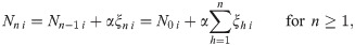
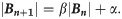
The standard Pólya urn (see [49–51]) is a stochastic model driven by a reinforcement mechanism (also known as “rich get richer” principle): the probability that a given event occurs increases with the number of times the same event occurred in the past. This rule is a key feature governing the dynamics of many biological, economic and social systems (see, e.g. [51]) and it seems plausible that it plays a role also in the sentiment dynamics of the Twitter posts as the emotional state of an individual influences the emotions of others [36, 52]. The Pólya urn model has been widely studied and generalized (some recent variants can be found in [48, 53–65]) and in its simplest form, with c-colors, works as follows. An urn contains N_0i balls of color i, for i = 1, …, c, and, at each discrete time-step, a ball is extracted from the urn and then it is returned inside the urn together with α > 0 additional balls of the same color. Therefore, if we denote by N_ni the number of balls of color i in the urn at time-step n, we have

2.2 Rescaled Pólya (RP) urn

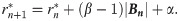
The “Rescaled” Pólya (RP) urn model, introduced in [48], is characterized by the introduction of the parameter β, together with the initial parameters (b_0i)_{i = 1, …, c} and (B_0i)_{i = 1, …, c}, next to the parameter α of the original model, so that

Therefore, the urn initially contains b_0i + B_0i > 0 balls of color i and the parameter β ≥ 0, together with α > 0, regulates the reinforcement mechanism. More precisely, the term βB_n−1i links N_ni to the “configuration” at time-step n − 1 through the “scaling” parameter β, and the term αξ_ni links N_ni to the outcome of the extraction at time-step n through the parameter α. Note that the case β = 1 corresponds to the standard Pólya urn with an initial number N_0i = b_0i + B_0i of balls of color i. When β ∈ [0, 1), this variant of the Pólya urn is characterized by a “local” reinforcement, i.e. a reinforcement mechanism mainly based on the most recent observations, and by a random persistent fluctuation of the predictive mean ψ_ni = E[ξ_n+1i = 1 |“past”]. As we will show, this latter feature is capable of capturing the trend fluctuations in the sentiment curve of Twitter posts (see Figs 1–6).

Fig 1

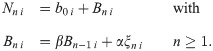
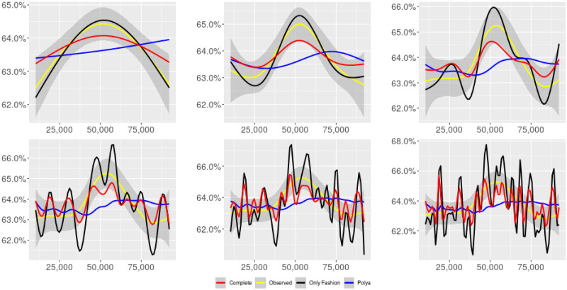
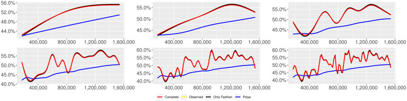
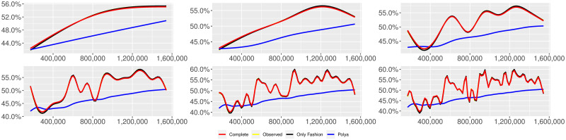
“Migration” (T = 0.35, entire, D = 3′, S = 100 slots of equal size): Sentiment curves.

In each panel, the yellow line is the cubic spline smoothing of the time series of the observed tweets ξ_n+1, together with the default confidence interval (gray), the red line represents the cubic spline smoothing of the time series of the estimated predictive means $$ {\widehat{\psi }}_n$$ (defined in Subsec. 3.2), obtained with the complete RP model, the black and the blue lines provide similar approximations obtained with the other models: black = Only fashion RP model and blue = Standard Pólya model. In each panel, the smoothing is obtained with a given number of nodes: k = 3 (top left panel), 5 (top middle panel), 10 (top right panel), 20 (bottom left panel), 30 (bottom middle panel), 50 (bottom right panel).

Fig 2

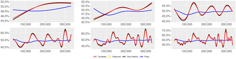
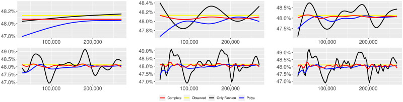
“Migration” (T = 0.35, only BOTs’ posts, D = 3′, S = 100 slots of equal size): Sentiment curves for BOTs’ posts.

In each panel, the yellow line is the cubic spline smoothing of the time series of the observed tweets ξ_n+1, together with the default confidence interval (gray), the red line represents the cubic spline smoothing of the time series of the estimated predictive means $$ {\widehat{\psi }}_n$$ (defined in Subsec. 3.2), obtained with the complete RP model, the black and the blue lines provide similar approximations obtained with the other models: black = Only fashion RP model and blue = Standard Pólya model. In each panel, the smoothing is obtained with a given number of nodes: k = 3 (top left panel), 5 (top middle panel), 10 (top right panel), 20 (bottom left panel), 30 (bottom middle panel), 50 (bottom right panel).

Fig 3

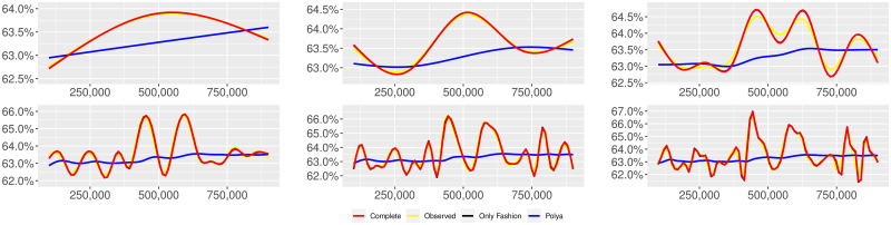
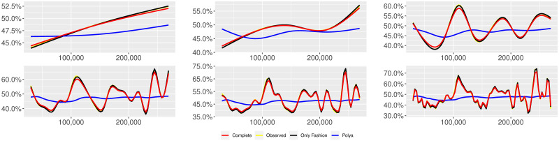
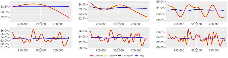
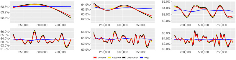
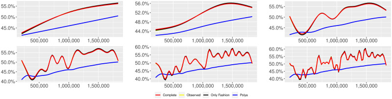
“10 days of traffic” (T = 0.35, entire, D = 30′′, S = 100 slots of equal size): Sentiment curves.

In each panel, the yellow line is the cubic spline smoothing of the time series of the observed tweets ξ_n+1, together with the default confidence interval (gray), the red line represents the cubic spline smoothing of the time series of the estimated predictive means $$ {\widehat{\psi }}_n$$ (defined in Subsec. 3.2), obtained with the complete RP model, the black and the blue lines provide similar approximations obtained with the other models: black = Only fashion RP model and blue = Standard Pólya model. In each panel, the smoothing is obtained with a given number of nodes: k = 3 (top left panel), 5 (top middle panel), 10 (top right panel), 20 (bottom left panel), 30 (bottom middle panel), 50 (bottom right panel).

Fig 4

“10 days of traffic” (T = 0.35, only BOTs’ posts, D = 30′′, S = 100 slots of equal size): Sentiment curves for BOTs’ postsx.

In each panel, the yellow line is the cubic spline smoothing of the time series of the observed tweets ξ_n+1, together with the default confidence interval (gray), the red line represents the cubic spline smoothing of the time series of the estimated predictive means $$ {\widehat{\psi }}_n$$ (defined in Subsec. 3.2), obtained with the complete RP model, the black and the blue lines provide similar approximations obtained with the other models: black = Only fashion RP model and blue = Standard Pólya model. In each panel, the smoothing is obtained with a given number of nodes: k = 3 (top left panel), 5 (top middle panel), 10 (top right panel), 20 (bottom left panel), 30 (bottom middle panel), 50 (bottom right panel).

Fig 5

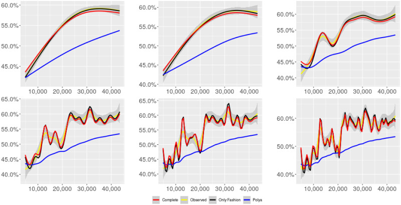
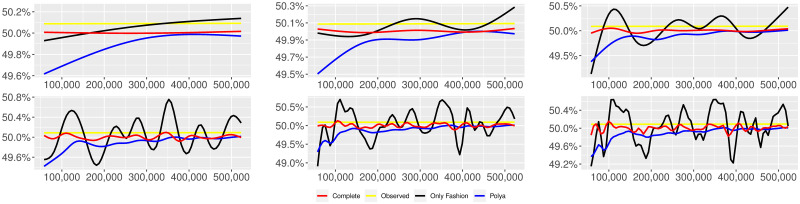
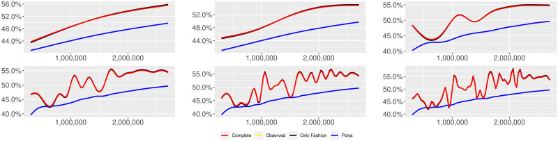
“Covid” (T = 0.35, entire, D = 3′, S = 1000 slots of equal size): Sentiment curves.

In each panel, the yellow line is the cubic spline smoothing of the time series of the observed tweets ξ_n+1, together with the default confidence interval (gray), the red line represents the cubic spline smoothing of the time series of the estimated predictive means $$ {\widehat{\psi }}_n$$ (defined in Subsec. 3.2), obtained with the complete RP model, the black and the blue lines provide similar approximations obtained with the other models: black = Only fashion RP model and blue = Standard Pólya model. In each panel, the smoothing is obtained with a given number of nodes: k = 3 (top left panel), 5 (top middle panel), 10 (top right panel), 20 (bottom left panel), 30 (bottom middle panel), 50 (bottom right panel).

Fig 6

“Covid” (T = 0.35, only BOTs’ posts, D′ = 3, S = 1000 slots of equal size): Sentiment curves for BOTs’ posts.

In each panel, the yellow line is the cubic spline smoothing of the time series of the observed tweets ξ_n+1, together with the default confidence interval (gray), the red line represents the cubic spline smoothing of the time series of the estimated predictive means $$ {\widehat{\psi }}_n$$ (defined in Subsec. 3.2), obtained with the complete RP model, the black and the blue lines provide similar approximations obtained with the other models: black = Only fashion RP model and blue = Standard Pólya model. In each panel, the smoothing is obtained with a given number of nodes: k = 3 (top left panel), 5 (top middle panel), 10 (top right panel), 20 (bottom left panel), 30 (bottom middle panel), 50 (bottom right panel).

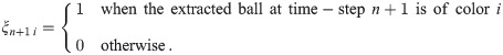
More formally, given a vector $$ \mathit{x}={(x_1,\dots ,x_c)}^{\top }\in {\mathbb{R}}^c$$, we define $$ \left|\mathit{x}\right|={\sum }_{i=1}^c\left|x_i\right|$$. Moreover, we set b₀ = (b₀₁, …, b_0c)^⊤ and B₀ = (B₀₁, …, B_0c)^⊤, we assume |b₀|>0 and we define $$ {\mathit{p}}_{\mathbf{0}}=\frac{{\mathit{b}}_{\mathbf{0}}}{|{\mathit{b}}_{\mathbf{0}}|}$$. At each discrete time-step (n + 1)≥1, a ball is drawn at random from the urn, obtaining the random vector ξ_n+1 = (ξ_n+11, …, ξ_n+1c)^⊤ defined as

The number of balls in the urn is so updated:

Therefore, setting $$ r_n^{*}=|{\mathit{N}}_{\mathit{n}}|=|{\mathit{b}}_{\mathbf{0}}|+|{\mathit{B}}_{\mathit{n}}|$$, we get

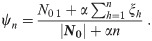
Moreover, denoting by $$ \mathcal{F}={\left({\mathcal{F}}_n\right)}_{n\ge 0}$$ the filtration representing the information along time-steps (formally, this means to set $$ {\mathcal{F}}_0$$ equal to the trivial σ-field and $$ {\mathcal{F}}_n=\sigma ({\mathit{\xi }}_{\mathbf{1}},\dots ,{\mathit{\xi }}_{\mathit{n}})$$ for n ≥ 1), the conditional probabilities ψ_n = (ψ_n1, …, ψ_nc)^⊤ of the extraction process, also called predictive means, are

This urn model has been studied in [48, 53]. All the mathematical proofs and details can be found in these papers.

2.2.1 Two colors (c = 2)

With two colors, the quantity of interest are only ξ_n = ξ_n1 = 1 − ξ_n2 and ψ_n = ψ_n1 = 1 − ψ_n2. In the sequel, we consider the RP urn model with β = 1 (i.e. the standard Pólya urn model) and with β < 1. In the first case, we have

In the second case, by (1), (2), (3) and (4), using $$ {\sum }_{m=0}^{n-1}{x}^m=(1-x^n)/(1-x)$$, we obtain

and

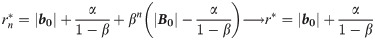
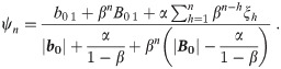
Since β < 1, the dependence of ψ_n on ξ_h exponentially increases with h, because of the factor β^n−h, and so the main contribution is given by the most recent extractions. We refer to this phenomenon as “local” reinforcement. The case β = 0 is an extreme case, for which ψ_n depends only on the last extraction ξ_n. Note that, when β = 1, i.e. the case of the standard Pólya urn, all the past observations ξ_h equally contribute to ψ_n, with a weight equal to α. This different dependence on the past leads to a different behaviour of ψ_n along time-steps (see [48]): in the standard Pólya urn, the process (ψ_n) asymptotically stabilizes, converging almost surely toward a random variable, while in the RP urn, the process (ψ_n) persistently fluctuates (see Figs 1–6).

If we set

we get for a large n

and

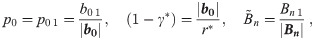
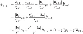
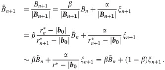
Summing up, the model dynamics can be approximated for n large by

where $$ p_0,{\gamma }^{*},\beta ,{\tilde{B}}_0$$ are the parameters. Note that α does not appear among the parameters for the above approximated dynamics, but it is included in the new parameter γ*. Moreover, the quantity $$ {\tilde{B}}_0$$ is exponentially fast negligible, because we have $$ {\tilde{B}}_n={\beta }^n{\tilde{B}}_0+(1-\beta ){\sum }_{h=1}^n{\beta }^{n-h}{\xi }_h$$, with β < 1. Therefore, the fundamental parameters are p₀, γ* and β: p₀ is a deterministic component, γ* tunes the weight in the predictive mean ψ_n+1 of the random “fluctuation” component $$ {\tilde{B}}_{n+1}$$ with respect to the deterministic one, and β regulates the dependence of the present state $$ {\tilde{B}}_{n+1}$$ on the previous state $$ {\tilde{B}}_n$$ and on the present observation ξ_n+1. We refer to $$ {\left({\tilde{B}}_n\right)}_n$$ as the “fashion” process, since it reproduces the trend variations of the considered phenomenon (in our case, the sentiment of Twitter posts). In the following applications, we consider the following cases:

Complete RP model: The three parameters θ = (p₀, γ*, β) are free to vary.

“Only Fashion” RP model: γ* = 1 (and p₀ = 0 irrelevant). This means that the predictive mean is not driven by any deterministic component, but it coincides with the fashion process. The free parameter is given by θ = β.

“No Fashion” RP model: γ* = 0 (and β = 0 irrelevant). In this case ψ_n is equal to the constant p₀ and, consequently, the free parameter is given by θ = p₀.

2.3 Model with delay

In applications, the extractions from the urn typically correspond to actions performed by agents. Therefore, it is plausible that there is a delay in information, in the sense that, when the agent decides to make the action that will appear at time-step n + 1, he/she only knows what happened until a certain time-step t(n)<n, i.e. the actions at time-steps 1, …, t(n). For instance, in our framework, the actions are the tweets and so it is plausible that, when the author of the tweet posted at time-step n + 1 is writing, he /she only knows the previous tweets until a certain time-step t(n)<n. In other words, we can image that an agent, after reading the tweets posted until time-step t(n), starts to write his/her tweet and posts it at time-step n + 1. Therefore, tweet n + 1 is not affected by tweets posted at time-steps t(n) + 1, …, n. When this is the case, the predictive means for action n + 1 are given by the composition of the urn until time-step t(n). In particular, if the number of colors is c = 2 and we denote by $$ {\mathcal{I}}_n$$ the information the agent has when performing action n + 1 (formally, $$ {\mathcal{I}}_0$$ equal to the trivial σ-field and $$ {\mathcal{I}}_n=\sigma ({\xi }_1,\dots ,{\xi }_{t\left(n\right)})$$), we have

Assuming to know the real time at which actions appeared (i.e., in our framework, the real time at which the posts are posted), a possible way to define t(n) is the following. Fix a value D > 0, divide (real) time in blocks of length D (choose D so that the blocks contain at least one action), define j(n + 1) the index of the time block containing the action n + 1 and set

It follows that, for all actions appeared in a certain time block j, the missing information are the actions appeared in the immediately previous time block (i.e. block j − 1) plus the preceding actions of the same block. As a consequence, the quantity D is a lower bound for the delay and 2D an upper bound: agents looses at least D units of time and not more than 2D units of time.

In the following, we refer to this variant of the RP urn as “RP urn model with delay”.

3.1 Data

Data have been collected from the Twitter platform, using the official API to Stream the exchange of messages on several topics. In the following, the various datasets are described in more details:

Italy, Migration debate

Data were collected through the Filter API since 23rd of January to 22nd of February 2019 and targeted the Italian debate on migration. Data were previously analysed in [16]. In the dataset, the information about the nature, automated or not (BOT or not), of the users is present. The BOT detection algorithm embedded is a lightweight version of the classifier proposed in [10]; more details on the dataset can be found in [16].

Italy, 10 days of traffic

The dataset collects the entire traffic, compatibly with the Filter API sampling, of messages in Italian in the days from the first to the 10th of September 2019: the keyword used for the query were the Italian vowels, in order to collect all messages that may contain some word. In the dataset, the information about the nature, automated or not (BOT or not), of the users is present. The BOT detection algorithm used was developed in [14].

Italy, COVID-19 epidemic

The dataset covers the period from February 21st to April to 20th 2020, including tweets in Italian language, and was previously analysed in [20]. The keywords used for the query are relative to the COVID-19 epidemic; more details can be found in the original reference. The dataset includes information on the automated or not (BOT or not) nature of the accounts, detected using the algorithm developed in [14].

For every message, the relative sentiment was calculated using the polyglot python module developed in [66], that provides a numerical value v ∈ [−1, 1] for the sentiment. We fix a threshold T = 0.35 so that we classify as a tweet with positive sentiment those with v > T and as a tweet with negative sentiment those with v < −T. We discard tweets with a value v ∈ [−T, T]. (There is not a particular reason for our choice of the value of T: indeed, we take the value 0.35 only because the interval [−1, 1] results divided into three parts of almost the same length. In Appendix, Sec. B, we show the results for other values of the threshold T).

Tables 1–3 show some descriptives of the samples obtained with T = 0.35:

Table 1

“Migration” sample: Descriptives of the sample obtained with T = 0.35.

Migration	Entire	Only BOTs’ posts
Posts	367367	4124
Percentage of positive posts	49.60%	47.97%

Table 2

“10 days of traffic” sample: Descriptives of the sample obtained with T = 0.35.

10 days of traffic	Entire	Only BOTs’ posts
Posts	3164620	102374
Percentage of positive posts	63.26%	63.79%

Table 3

“Covid” sample: Descriptives of the sample obtained with T = 0.35.

Covid	Entire	Only BOTs’ posts
Posts	2037584	48252
Percentage of positive posts	50.58%	54.00%

3.2 Analysis of the prediction ability

We apply the RP urn model with delay, ordering the tweets according to their creation time and taking each tweet with a positive/negative classification as an extraction in the urn model. More precisely, we apply the RP model with c = 2: the time series of the tweets represents the time series of the extractions from the urn, that is the random variables ξ_n. The event {ξ_n = 1} means that tweet n exhibits a positive sentiment, while {ξ_n = 0} means that tweet n exhibits a negative sentiment. Moreover, we include a delay into the model as described in Subsec. 2.3, taking D = 3 minutes for the “migration” and “covid” samples and D = 30 seconds for the “10 days of traffic” sample. These values have been arbitrarily chosen, because we have no information about the real length of the delay. Notably, no significant difference has been observed taking zero delay.

The model parameters have been estimated by maximum likelihood. More precisely, we have divided the available N (ordered) actions (i.e. the tweets) into S slots of the same size (numbered from s = 0 to s = S − 1). For each slot s = 1, …, S − 1, with training data of the slots s′ = 0, …, s − 1, we have estimated the best parameters $$ \widehat{\theta }\left(s\right)$$ for the different proposed models (with delay): Standard Pólya, Complete RP, Only Fashion RP, No Fashion RP. (See Appendix, Sec. A, for a deeper exploration of the evolution of the parameters and further comments.) With these parameters, for each action ξ_n+1 of the s-th slot, we have computed the conditional probability $$ {\widehat{\psi }}_n$$ (see Eq 5), that is the predictive mean for action n + 1, as a function of the estimated parameters and of the actions ξ₁, …, ξ_t(n) (that is the information of the author of action n + 1). The predictive mean $$ {\widehat{\psi }}_n$$ represents our prediction of the future action ξ_n+1. We have quantified the ability of the considered model to predict the future outcomes by means of the relative Squared Error (SE_rel) with respect to the method that predicts the future outcome taking the value assumed by the majority in the past. More precisely, we have computed the following quantity:

This quantity measures the ability of the model to predict the future outcomes: the greater it is, the better is the prediction with respect to the method based on the past majority. The values SE_rel obtained for the different considered models are also compared with the “theoretical” value of SE_rel computed replacing $$ {\widehat{\psi }}_n$$ by the mean value $$ \overline{\psi }$$ on all the considered period. The term “theoretical” is used in order to point out that $$ \overline{\psi }$$ is of course not a prediction, but it gives the a posteriori best constant fit once we have collected all the data until time-step N. Summing up, our aim is twofold: to obtain a value of SE_rel greater than 1, that means that the considered models beat the performance of the method based on the past majority, and to get a value greater or equal to the “theoretical” value, that means that the proposed models perform better or similarly than the (theoretical) a posteriori best constant fit.

We summarize the results in Tables 4–6. For each considered sample, we have also analysed the subset obtained by the restriction to the tweets classified as sent by a BOT. In the tables the best values are highlighted in bold. We can observe that, for the “Migration” and “covid” samples, the considered models perform more or less two times better than the method based on the past majority and this performance is similar to (indeed, in the most cases slightly better than) the one given by the (theoretical) a posteriori best constant fit. For the “10 days traffic” sample, the performance of the considered models is one and half times better than the method based on the past majority and this performance is similar to the one given by the (theoretical) a posteriori best constant fit. Moreover, the performances of the “Complete RP” model and of the “Only fashion RP” model do not significantly differ; while the “No Fashion RP” model performs less well. Therefore, in the next subsection, we will discard this last model.

Table 4

“Migration” sample (T = 0.35, D = 3′, S = 100 slots of equal size): Comparison of the different considered models in terms of (6).

Migration	Standard Pólya	Complete RP	Only Fashion RP	No Fashion RP	Theoretical value
Entire	200.91%	206.28%	206.22%	200.78%	200.93%
OnlyBOT	194.52%	199.63%	199.75%	194.24%	194.74%

Table 5

“10 days of traffic” sample (T = 0.35, D = 30′′, S = 100 slots of equal size): Comparison of the different considered models in terms of (6).

10 days of traffic	Standard Pólya	Complete RP	Only Fashion RP	No Fashion RP	Theoretical value
Entire	160.75%	160.88%	160.88%	160.74%	160.75%
OnlyBOT	159.57%	159.70%	159.62%	159.57%	159.58%

Table 6

“Covid” sample (T = 0.35, D = 3′, S = 1000 slots of equal size): Comparison of the different considered models in terms of (6).

Covid	Standard Pólya	Complete RP	Only Fashion RP	No Fashion RP	Theoretical value
Entire	199.97%	203.15%	203.15%	199.96%	200.02%
OnlyBOT	187.60%	190.43%	190.47%	187.58%	187.85%

(In Appendix, Sec. B, we collect results obtained with different thresholds T (used for the construction of the sample) and taking the slots (used for the parameters estimation) equal to the available days of observation).

3.3 Fluctuations of the sentiment curve

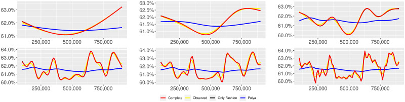
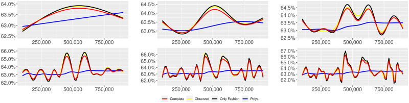
We provide some tables and figures in order to point out how the different considered models are able to reproduce the trend fluctuation of the sentiment curve. More precisely, in Figs 1–6, the yellow line is the cubic spline smoothing (Penalized Cubic regression splines with different numbers of nodes: k = 3, 5, 10, 20, 30, 50. See [67]) of the time series of the observed tweets {ξ_n: n = 1, …, N}, together with the default confidence interval (gray), the red line represents the cubic spline smoothing (with the same number of nodes) of the time series of the estimated predictive means $$ {\widehat{\psi }}_n$$ (see Subsec. 3.2), obtained with the complete RP model with delay, the black and the blue lines provide similar approximations obtained with the other models with delay: black = Only fashion RP model and blue = Standard Pólya model. In Tables 7–12, we compare the different models by means of the Mean Squared Error (MSE), i.e.

Table 7

“Migration” (T = 0.35, entire, D = 3′, S = 100 slots of equal size): MSE for different levels of smoothing.

smoothing	Only Fashion RP	Complete RP	Standard Pólya
no smooth	2.44 × 10−1	2.43 × 10−1	2.50 × 10−1
k = 3	3.44 × 10−9	1.41 × 10−6	3.03 × 10−4
k = 5	1.19 × 10−8	3.23 × 10−6	3.43 × 10−4
k = 10	2.64 × 10−7	1.74 × 10−5	1.64 × 10−3
k = 20	1.04 × 10−6	2.98 × 10−5	2.73 × 10−3
k = 30	2.79 × 10−6	4.03 × 10−5	3.83 × 10−3
k = 50	7.18 × 10−6	5.41 × 10−5	4.85 × 10−3

Table 8

“Migration” (T = 0.35, only BOTs’ posts, D = 3′, S = 100 slots of equal size): MSE for different levels of smoothing.

smoothing	Only Fashion RP	Complete RP	Standard Pólya
no smooth	2.43 × 10−1	2.41 × 10−1	2.50 × 10−1
k = 3	2.62 × 10−6	3.56 × 10−5	7.66 × 10−4
k = 5	4.19 × 10−4	1.90 × 10−4	1.10 × 10−3
k = 10	1.03 × 10−4	3.50 × 10−4	3.36 × 10−3
k = 20	5.36 × 10−4	8.19 × 10−4	6.58 × 10−3
k = 30	9.09 × 10−4	1.22 × 10−3	9.13 × 10−3
k = 50	2.53 × 10−3	2.36 × 10−3	1.34 × 10−2

Table 9

“10 days of traffic” (T = 0.35, entire, D = 30′′, S = 100 slots of equal size): MSE for different levels of smoothing.

smoothing	Only Fashion RP	Complete RP	Standard Pólya
no smooth	2.32 × 10−1	2.32 × 10−1	2.33 × 10−1
k = 3	3.15 × 10−9	2.61 × 10−7	1.22 × 10−5
k = 5	3.86 × 10−9	8.09 × 10−7	3.34 × 10−5
k = 10	1.94 × 10−8	2.02 × 10−6	6.88 × 10−5
k = 20	7.81 × 10−8	2.65 × 10−6	8.80 × 10−5
k = 30	1.74 × 10−7	2.86 × 10−6	9.65 × 10−5
k = 50	1.08 × 10−6	5.15 × 10−6	1.53 × 10−4

Table 10

“10 days traffic” (T = 0.35, only BOTs’ posts, D = 30′′, S = 100 slots of equal size): MSE for different levels of smoothing.

smoothing	Only Fashion RP	Complete RP	Standard Pólya
no smooth	2.31 × 10−1	2.31 × 10−1	2.31 × 10−1
k = 3	4.10 × 10−7	6.67 × 10−7	5.73 × 10−6
k = 5	7.95 × 10−7	2.02 × 10−5	5.97 × 10−5
k = 10	6.81 × 10−6	2.35 × 10−5	7.19 × 10−5
k = 20	1.59 × 10−5	5.43 × 10−5	1.52 × 10−4
k = 30	2.59 × 10−5	5.98 × 10−5	1.75 × 10−4
k = 50	9.80 × 10−5	1.23 × 10−4	3.49 × 10−4

Table 11

“Covid” (T = 0.35, entire, D = 3′, S = 1000 slots of equal size): MSE for different levels of smoothing.

smoothing	Only Fashion RP	Complete RP	Standard Pólya
no smooth	2.46 × 10−1	2.46 × 10−1	2.50 × 10−1
k = 3	3.98 × 10−8	7.37 × 10−6	2.58 × 10−3
k = 5	5.51 × 10−8	7.53 × 10−6	2.64 × 10−3
k = 10	1.54 × 10−7	8.63 × 10−6	2.92 × 10−3
k = 20	7.93 × 10−7	9.37 × 10−6	3.10 × 10−3
k = 30	1.06 × 10−6	9.80 × 10−6	3.24 × 10−3
k = 50	2.06 × 10−6	1.10 × 10−5	3.46 × 10−3

Table 12

“Covid” (T = 0.35, only BOTs’ posts, D = 3′, S = 1000 slots of equal size): MSE for different levels of smoothing).

smoothing	Only Fashion RP	Complete RP	Standard Pólya
no smooth	2.45 × 10−1	2.45 × 10−1	2.49 × 10−1
k = 3	3.23 × 10−6	5.33 × 10−5	3.38 × 10−3
k = 5	1.16 × 10−5	5.16 × 10−5	3.38 × 10−3
k = 10	2.84 × 10−5	6.88 × 10−5	3.53 × 10−3
k = 20	5.70 × 10−5	9.78 × 10−5	3.80 × 10−3
k = 30	1.67 × 10−4	1.81 × 10−4	4.01 × 10−3
k = 50	3.05 × 10−4	2.94 × 10−4	4.38 × 10−3

We can observe that, as explained before in Section 2.2, the RP urn model is able to reproduce the fluctuations of the observed sentiment curve, while the standard Pólya urn model produces a curve that converges to a value.

(In Appendix, Sec. B, we collect results obtained with different thresholds T (used for the construction of the sample) and taking the slots (used for the parameters estimation described in Subsec. 3.2) equal to the available days of observation).

A Parameters evolution

As it is mentioned in the main text, in order to fit the parameters of the model, we divided the entire sample in slots of the same size (the number S of slots and their size for each considered sample is specified in the captions of the figures). Next, we use all slots previous to the one under consideration to fit the parameters. In this sense, we observe an evolution of the parameters as a matter of the evolution of the samples, which is different when focusing on the different nature of users in the debate. Such a difference is particularly evident in the Migration debate. Human accounts show a nearly constant parameter dynamics: while β is nearly constant in the Complete model, γ* and p₀ display a smooth slow variation of nearly the 10% of their value, see Fig 7. The dynamics of the parameters for automated accounts is completely different, see Fig 8: in the Complete model, while β is slowly decreasing (but still experiencing a much greater decrease than the one observed for human accounts), parameters γ* and p₀ display a step-like dynamics, ending shortly after s = 25.

Fig 7

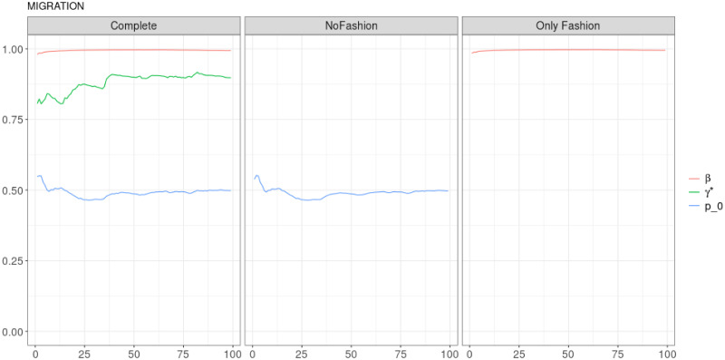
“Migration” (T = 0.35, entire, D = 3′): Model parameters evolution with S = 100 slots of equal size (i.e. 3673 observations).

All parameters are slowly varying and converging to stable values.

Fig 8

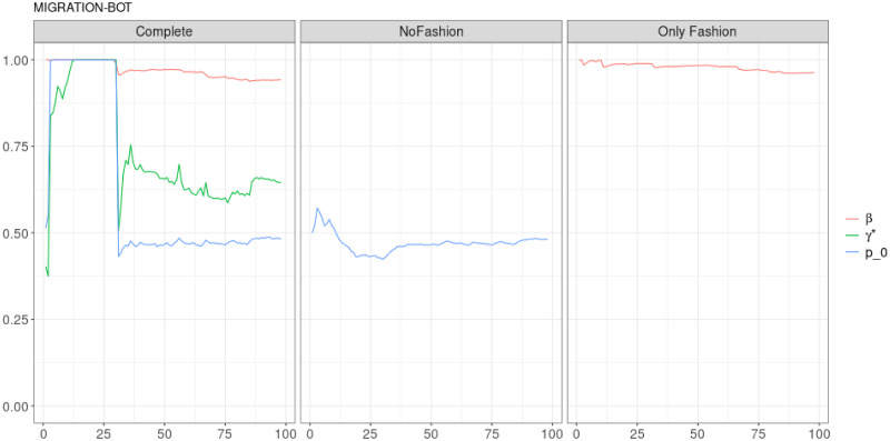
“Migration” (T = 0.35, only BOTs’ posts, D = 3′): Model parameters evolution with S = 100 slots of equal size (i.e. 41 observations).

In the left panel, it is possible to distinguish an “Only fashion” initial phase (γ* ≃ 1) and more balanced phase (γ* ∈ [0.5, 0.75]).

A similar, but less evident, dynamics can be observed in the “10 days of traffic” sample, see Figs 9 and 10: in this case, all parameters converge to 1 quite soon in the case of the entire sample. Instead, we can see that p₀ converge, but to something more than 0.6 quite immediately for the social bot subset, while the value of γ* oscillates between 0.5 and 0, before converging to something less than 0.4. The parameter β is nearly 1 for both cases.

Fig 9

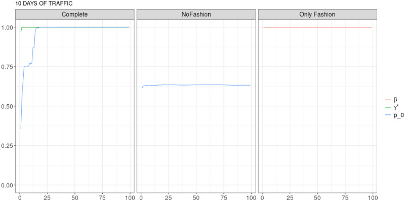
“10 days of traffic” (T = 0.35, entire, D = 30′′): Model parameters evolution with S = 100 slots of equal size (i.e. 31646 observations).

All parameters for the complete model converge to 1 quite soon. With γ* ≃ 1, the Complete model is practically equivalent to the “Only Fashion” one.

Fig 10

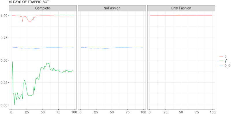
“10 days of traffic” (T = 0.35, only BOTs’ posts, D = 30′′): Model parameters evolution with S = 100 slots of equal size (i.e. 1023 observations).

Every parameter of the complete model, but γ*, are essentially constant. Let us remark that γ* tunes the weight of the fashion process in the predictive mean.

In the case of the online debate during the COVID-19 epidemic, Figs 11 and 12, the differences are extremely low, with the values of γ* quite flickering before converging to a value little lower than the one obtained for the entire sample. All other parameters are quite similar, both in the value and in the dynamics.

Fig 11

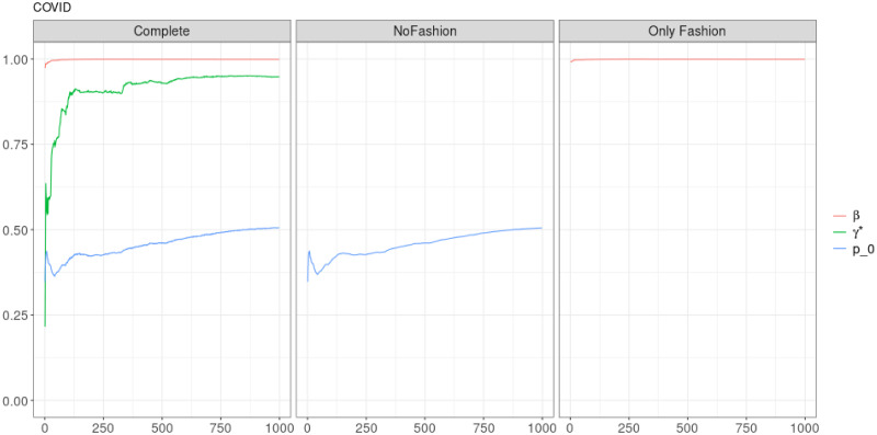
“Covid” (T = 0.35, entire, D = 3′): Model parameters evolution with S = 1000 slots of equal size (i.e. 2037 observations).

All parameters are nearly constant or slowly converging.

Fig 12

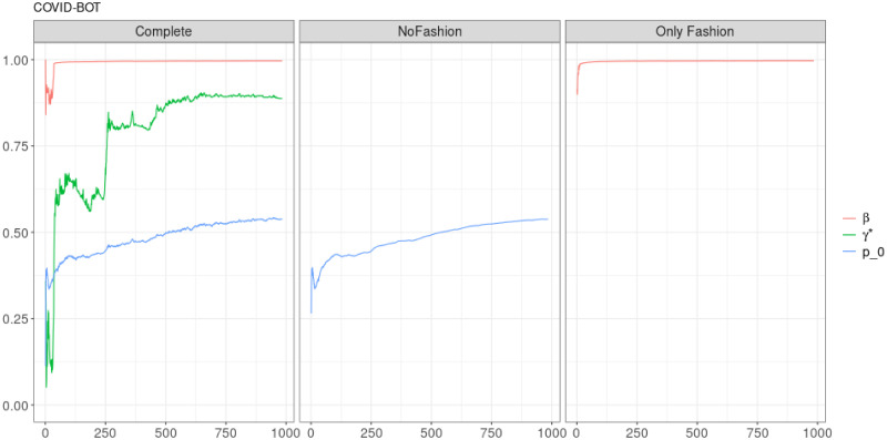
“Covid” (T = 0.35, only BOTs’ posts, D = 3′): Model parameters evolution with S = 1000 slots of equal size (i.e. 48 observations).

Differently to the other samples, the parameters evolution for the Bots’ posts follows the one for the entire sample, displaying a greater noise contribution for γ*.

It is worthwhile to point out that, when we deal with the entire samples, the size of each slot is large enough in order to estimate properly the parameters from the very beginning. Therefore, we can guess that the behaviours of the curves in Figs 7, 9 and 11, before the stabilization, are really related to the dynamics of the debates. The situation is different when we deal only with posts sent by BOTs. Indeed, in this case, the initial estimation of the parameters may be affected by the limited size of the slots. However, also Figs 8, 10 and 12 exhibits a final stabilization of the values. An open question is if the differences in the values of the parameters and in their long-term dynamics observed when comparing the entire sample and the subset of BOTs’ posts is due to the different sizes or to an indeed different dynamics. This issue is not the focus of this work and it is going to be the target of further analyses.

B Additional analyses

We here collect the outputs of some additional analyses related to different choices of the threshold T for the construction of the sample and to a different partition into slots associated to the applied estimation technique for the model parameters. More precisely, we perform the analyses described in Subsecs. 3.2 and 3.3 for other two different thresholds (i.e. T = 0.5 and T = 0) and also taking the slots equal to the available days of observation. Table 13 reports the values of the indicator defined in Subsec. 3.2, Eq (6). Tables 14–25 and Figs 13–24 illustrate the results of the analyses described in Subsec. 3.3. We can observe that the main finding of this work does not change: indeed, since its local reinforcement mechanism, the RP urn model (with delay) is able to reproduce the fluctuations of the observed sentiment curve.

Fig 13

“Migration” (T = 0.5, entire, D = 3′, S = 100 slots of equal size): Sentiment curves.

In each panel, the yellow line is the cubic spline smoothing of the time series of the observed tweets ξ_n+1, together with the default confidence interval (gray), the red line represents the cubic spline smoothing of the time series of the estimated predictive means $$ {\widehat{\psi }}_n$$ (defined in Subsec. 3.2), obtained with the complete RP model, the black and the blue lines provide similar approximations obtained with the other models: black = Only fashion RP model and blue = Standard Pólya model. In each panel, the smoothing is obtained with a given number of nodes: k = 3 (top left panel), 5 (top middle panel), 10 (top right panel), 20 (bottom left panel), 30 (bottom middle panel), 50 (bottom right panel).

Fig 14

“Migration” (T = 0, entire, D = 3′, S = 100 slots of equal size): Sentiment curves.

In each panel, the yellow line is the cubic spline smoothing of the time series of the observed tweets ξ_n+1, together with the default confidence interval (gray), the red line represents the cubic spline smoothing of the time series of the estimated predictive means $$ {\widehat{\psi }}_n$$ (defined in Subsec. 3.2), obtained with the complete RP model, the black and the blue lines provide similar approximations obtained with the other models: black = Only fashion RP model and blue = Standard Pólya model. In each panel, the smoothing is obtained with a given number of nodes: k = 3 (top left panel), 5 (top middle panel), 10 (top right panel), 20 (bottom left panel), 30 (bottom middle panel), 50 (bottom right panel).

Fig 15

“Migration” (T = 0.35, entire, D = 3′, slots = days): Sentiment curves.

In each panel, the yellow line is the cubic spline smoothing of the time series of the observed tweets ξ_n+1, together with the default confidence interval (gray), the red line represents the cubic spline smoothing of the time series of the estimated predictive means $$ {\widehat{\psi }}_n$$ (defined in Subsec. 3.2), obtained with the complete RP model, the black and the blue lines provide similar approximations obtained with the other models: black = Only fashion RP model and blue = Standard Pólya model. In each panel, the smoothing is obtained with a given number of nodes: k = 3 (top left panel), 5 (top middle panel), 10 (top right panel), 20 (bottom left panel), 30 (bottom middle panel), 50 (bottom right panel).

Fig 16

“Migration” (T = 0.5, entire, D = 3′, slots = days): Sentiment curves.

In each panel, the yellow line is the cubic spline smoothing of the time series of the observed tweets ξ_n+1, together with the default confidence interval (gray), the red line represents the cubic spline smoothing of the time series of the estimated predictive means $$ {\widehat{\psi }}_n$$ (defined in Subsec. 3.2), obtained with the complete RP model, the black and the blue lines provide similar approximations obtained with the other models: black = Only fashion RP model and blue = Standard Pólya model. In each panel, the smoothing is obtained with a given number of nodes: k = 3 (top left panel), 5 (top middle panel), 10 (top right panel), 20 (bottom left panel), 30 (bottom middle panel), 50 (bottom right panel).

Fig 17

“10 days of traffic” (T = 0.5, entire, D = 30′′, S = 100 slots of equal size): Sentiment curves.

In each panel, the yellow line is the cubic spline smoothing of the time series of the observed tweets ξ_n+1, together with the default confidence interval (gray), the red line represents the cubic spline smoothing of the time series of the estimated predictive means $$ {\widehat{\psi }}_n$$ (defined in Subsec. 3.2), obtained with the complete RP model, the black and the blue lines provide similar approximations obtained with the other models: black = Only fashion RP model and blue = Standard Pólya model. In each panel, the smoothing is obtained with a given number of nodes: k = 3 (top left panel), 5 (top middle panel), 10 (top right panel), 20 (bottom left panel), 30 (bottom middle panel), 50 (bottom right panel).

Fig 18

“10 days of traffic” (T = 0, entire, D = 30′′, S = 100 slots of equal size): Sentiment curves.

In each panel, the yellow line is the cubic spline smoothing of the time series of the observed tweets ξ_n+1, together with the default confidence interval (gray), the red line represents the cubic spline smoothing of the time series of the estimated predictive means $$ {\widehat{\psi }}_n$$ (defined in Subsec. 3.2), obtained with the complete RP model, the black and the blue lines provide similar approximations obtained with the other models: black = Only fashion RP model and blue = Standard Pólya model. In each panel, the smoothing is obtained with a given number of nodes: k = 3 (top left panel), 5 (top middle panel), 10 (top right panel), 20 (bottom left panel), 30 (bottom middle panel), 50 (bottom right panel).

Fig 19

“10 days of traffic” (T = 0.35, entire, D = 30′′, slots = days): Sentiment curves.

In each panel, the yellow line is the cubic spline smoothing of the time series of the observed tweets ξ_n+1, together with the default confidence interval (gray), the red line represents the cubic spline smoothing of the time series of the estimated predictive means $$ {\widehat{\psi }}_n$$ (defined in Subsec. 3.2), obtained with the complete RP model, the black and the blue lines provide similar approximations obtained with the other models: black = Only fashion RP model and blue = Standard Pólya model. In each panel, the smoothing is obtained with a given number of nodes: k = 3 (top left panel), 5 (top middle panel), 10 (top right panel), 20 (bottom left panel), 30 (bottom middle panel), 50 (bottom right panel).

Fig 20

“10 days of traffic” (T = 0.5, entire, D = 30′′y, slots = days): Sentiment curves.

In each panel, the yellow line is the cubic spline smoothing of the time series of the observed tweets ξ_n+1, together with the default confidence interval (gray), the red line represents the cubic spline smoothing of the time series of the estimated predictive means $$ {\widehat{\psi }}_n$$ (defined in Subsec. 3.2), obtained with the complete RP model, the black and the blue lines provide similar approximations obtained with the other models: black = Only fashion RP model and blue = Standard Pólya model. In each panel, the smoothing is obtained with a given number of nodes: k = 3 (top left panel), 5 (top middle panel), 10 (top right panel), 20 (bottom left panel), 30 (bottom middle panel), 50 (bottom right panel).

Fig 21

“Covid” (T = 0.5, entire, *D = 3′, S = 100 slots of equal size): Sentiment curves.

In each panel, the yellow line is the cubic spline smoothing of the time series of the observed tweets ξ_n+1, together with the default confidence interval (gray), the red line represents the cubic spline smoothing of the time series of the estimated predictive means $$ {\widehat{\psi }}_n$$ (defined in Subsec. 3.2), obtained with the complete RP model, the black and the blue lines provide similar approximations obtained with the other models: black = Only fashion RP model and blue = Standard Pólya model. In each panel, the smoothing is obtained with a given number of nodes: k = 3 (top left panel), 5 (top middle panel), 10 (top right panel), 20 (bottom left panel), 30 (bottom middle panel), 50 (bottom right panel).

Fig 22

“Covid” (T = 0, entire, D = 3′, S = 100 slots of equal size): Sentiment curves.

In each panel, the yellow line is the cubic spline smoothing of the time series of the observed tweets ξ_n+1, together with the default confidence interval (gray), the red line represents the cubic spline smoothing of the time series of the estimated predictive means $$ {\widehat{\psi }}_n$$ (defined in Subsec. 3.2), obtained with the complete RP model, the black and the blue lines provide similar approximations obtained with the other models: black = Only fashion RP model and blue = Standard Pólya model. In each panel, the smoothing is obtained with a given number of nodes: k = 3 (top left panel), 5 (top middle panel), 10 (top right panel), 20 (bottom left panel), 30 (bottom middle panel), 50 (bottom right panel).

Fig 23

“Covid” (T = 0.35, entire, D = 3′, slots = days): Sentiment curves.

In each panel, the yellow line is the cubic spline smoothing of the time series of the observed tweets ξ_n+1, together with the default confidence interval (gray), the red line represents the cubic spline smoothing of the time series of the estimated predictive means $$ {\widehat{\psi }}_n$$ (defined in Subsec. 3.2), obtained with the complete RP model, the black and the blue lines provide similar approximations obtained with the other models: black = Only fashion RP model and blue = Standard Pólya model. In each panel, the smoothing is obtained with a given number of nodes: k = 3 (top left panel), 5 (top middle panel), 10 (top right panel), 20 (bottom left panel), 30 (bottom middle panel), 50 (bottom right panel).

Fig 24

“Covid” (T = 0.5, entire, D = 3′, slots = days): Sentiment curves.

In each panel, the yellow line is the cubic spline smoothing of the time series of the observed tweets ξ_n+1, together with the default confidence interval (gray), the red line represents the cubic spline smoothing of the time series of the estimated predictive means $$ {\widehat{\psi }}_n$$ (defined in Subsec. 3.2), obtained with the complete RP model, the black and the blue lines provide similar approximations obtained with the other models: black = Only fashion RP model and blue = Standard Pólya model. In each panel, the smoothing is obtained with a given number of nodes: k = 3 (top left panel), 5 (top middle panel), 10 (top right panel), 20 (bottom left panel), 30 (bottom middle panel), 50 (bottom right panel).

Table 13

Comparison of the different considered models in terms of (6).

Sample	Standard Pólya	Complete RP	Only Fashion RP	No Fashion RP	Theoretical value
Migration (T = 0, D = 3’, S = 100)	202.23%	202.25%	202.22%	202.22%	202.23%
Migration (T = 0.5, D = 3’, S = 100)	194.48%	194.51%	194.48%	194.48%	194.48%
Migration (T = 0.35, D = 3’, slots = days)	198.84%	203.11%	203.46%	198.02%	198.86%
Migration (T = 0.5, D = 3’, slots = days)	192.67%	198.40%	198.78%	191.10%	192.70%
10 days traffic (T = 0, D = 30”, S = 100)	165.68%	165.79%	165.79%	165.68%	165.68%
10 days traffic (T = 0.5, D = 30”, S = 100)	160.18%	160.32%	160.32%	160.17%	160.18%
10 days traffic (T = 0.35, D = 30”, slots = days)	158.10%	158.23%	158.23%	158.08%	158.10%
10 days traffic (T = 0.5, D = 30”, slots = days)	157.50%	157.64%	157.64%	157.48%	157.50%
Covid (T = 0, D = 3’, S = 100)	201.60%	204.33%	204.33%	201.51%	201.70%
Covid (T = 0.5, D = 3’, S = 100)	199.04%	202.24%	202.25%	198.91%	199.10%
Covid (T = 0.35, D = 3’, slots = days)	198.01%	201.08%	201.11%	197.82%	198.01%
Covid (T = 0.5, D = 3’, slots = days)	197.10%	200.20%	200.23%	196.85%	197.10%

Table 14

“Migration” (T = 0.5, entire, D = 3′, S = 100 slots of equal size): MSE for different levels of smoothing.

smoothing	Only Fashion RP	Complete RP	Standard Pólya
no smooth	2.50 × 10−1	2.50 × 10−1	2.50 × 10−1
k = 3	3.58 × 10−7	5.37 × 10−7	5.79 × 10−6
k = 5	4.13 × 10−7	5.36 × 10−7	8.22 × 10−6
k = 10	9.97 × 10−6	6.04 × 10−7	9.65 × 10−6
k = 20	1.10 × 10−5	2.11 × 10−5	2.91 × 10−5
k = 30	2.29 × 10−5	3.48 × 10−5	4.36 × 10−5
k = 50	3.44 × 10−5	4.51 × 10−5	5.73 × 10−5

Table 15

“Migration” (T = 0, entire, D = 3′, S = 100 slots of equal size): MSE for different levels of smoothing.

smoothing	Only Fashion RP	Complete RP	Standard Pólya
no smooth	2.50 × 10−1	2.50 × 10−1	2.50 × 10−1
k = 3	1.96 × 10−8	1.20 × 10−6	3.31 × 10−6
k = 5	1.77 × 10−7	9.52 × 10−7	4.03 × 10−6
k = 10	3.70 × 10−6	9.94 × 10−7	4.20 × 10−6
k = 20	4.29 × 10−6	7.86 × 10−6	1.12 × 10−5
k = 30	5.79 × 10−6	9.84 × 10−6	1.37 × 10−5
k = 50	1.26 × 10−5	1.79 × 10−5	2.36 × 10−5

Table 16

“Migration” (T = 0.35, entire, D = 3′, slots = days): MSE for different levels of smoothing.

smoothing	Only Fashion RP	Complete RP	Standard Pólya
no smooth	2.44 × 10−1	2.44 × 10−1	2.50 × 10−1
k = 3	7.26 × 10−8	1.76 × 10−6	3.01 × 10−4
k = 5	1.10 × 10−7	4.16 × 10−6	3.43 × 10−4
k = 10	1.24 × 10−6	2.84 × 10−5	1.64 × 10−3
k = 20	5.41 × 10−6	5.01 × 10−5	2.74 × 10−3
k = 30	1.20 × 10−5	6.92 × 10−5	3.84 × 10−3
k = 50	2.59 × 10−5	9.73 × 10−5	4.87 × 10−3

Table 17

“Migration” (T = 0.5, entire, D = 3′, slots = days): MSE for different levels of smoothing.

smoothing	Only Fashion RP	Complete RP	Standard Pólya
no smooth	2.42 × 10−1	2.42 × 10−1	2.50 × 10−1
k = 3	2.66 × 10−7	2.29 × 10−6	3.56 × 10−4
k = 5	6.47 × 10−7	2.49 × 10−6	3.75 × 10−4
k = 10	2.75 × 10−6	3.75 × 10−5	2.79 × 10−3
k = 20	6.37 × 10−6	5.80 × 10−5	3.92 × 10−3
k = 30	1.66 × 10−5	8.32 × 10−5	5.33 × 10−3
k = 50	3.15 × 10−5	1.09 × 10−4	6.54 × 10−3

Table 18

“10 days of traffic” (T = 0.5, entire, D = 30′′, S = 100 slots of equal size): MSE for different levels of smoothing.

smoothing	Only Fashion RP	Complete RP	Standard Pólya
no smooth	2.32 × 10−1	2.32 × 10−1	2.32 × 10−1
k = 3	4.32 × 10−8	4.49 × 10−8	7.88 × 10−6
k = 5	5.40 × 10−9	6.29 × 10−9	5.56 × 10−5
k = 10	1.43 × 10−8	1.70 × 10−8	7.56 × 10−5
k = 20	6.65 × 10−8	8.04 × 10−8	9.78 × 10−5
k = 30	2.62 × 10−7	2.89 × 10−7	1.04 × 10−4
k = 50	1.00 × 10−6	1.20 × 10−6	1.53 × 10−4

Table 19

“10 days of traffic” (T = 0, entire, D = 30′′, S = 100 slots of equal size): MSE for different levels of smoothing.

smoothing	Only Fashion RP	Complete RP	Standard Pólya
no smooth	2.37 × 10−1	2.37 × 10−1	2.37 × 10−1
k = 3	6.56 × 10−9	5.77 × 10−9	3.68 × 10−5
k = 5	7.12 × 10−9	5.97 × 10−9	5.20 × 10−5
k = 10	1.86 × 10−8	1.62 × 10−8	6.71 × 10−5
k = 20	7.66 × 10−8	6.46 × 10−8	7.92 × 10−5
k = 30	2.69 × 10−7	2.44 × 10−7	8.49 × 10−5
k = 50	1.23 × 10−6	1.02 × 10−6	1.25 × 10−4

Table 20

“10 days of traffic” (T = 0.35, entire, D = 30′′, slots = days): MSE for different levels of smoothing.

smoothing	Only Fashion RP	Complete RP	Standard Pólya
no smooth	2.32 × 10−1	2.32 × 10−1	2.33 × 10−1
k = 3	3.15 × 10−9	2.63 × 10−7	1.22 × 10−5
k = 5	3.86 × 10−9	8.15 × 10−7	3.34 × 10−5
k = 10	1.94 × 10−8	2.03 × 10−6	6.88 × 10−5
k = 20	7.81 × 10−8	2.68 × 10−6	8.80 × 10−5
k = 30	1.74 × 10−7	2.88 × 10−6	9.65 × 10−5
k = 50	1.08 × 10−6	5.19 × 10−6	1.53 × 10−4

Table 21

“10 days of traffic” (T = 0.5, entire, D = 30′′, slots = days): MSE for different levels of smoothing.

smoothing	Only Fashion RP	Complete RP	Standard Pólya
no smooth	2.32 × 10−1	2.32 × 10−1	2.32 × 10−1
k = 3	4.32 × 10−8	1.62 × 10−7	7.88 × 10−6
k = 5	5.40 × 10−9	1.94 × 10−6	5.56 × 10−5
k = 10	1.43 × 10−8	2.71 × 10−6	7.56 × 10−5
k = 20	6.65 × 10−8	3.65 × 10−6	9.78 × 10−5
k = 30	2.62 × 10−7	3.58 × 10−6	1.04 × 10−4
k = 50	1.00 × 10−6	5.86 × 10−6	1.53 × 10−4

Table 22

“Covid” (T = 0.5, entire, D = 3′, S = 100 slots of equal size): MSE for different levels of smoothing.

smoothing	Only Fashion RP	Complete RP	Standard Pólya
no smooth	2.46 × 10−1	2.46 × 10−1	2.50 × 10−1
k = 3	4.50 × 10−8	8.40 × 10−6	2.37 × 10−3
k = 5	5.77 × 10−8	8.51 × 10−6	2.42 × 10−3
k = 10	1.39 × 10−7	1.03 × 10−5	2.84 × 10−3
k = 20	1.14 × 10−6	1.19 × 10−5	3.12 × 10−3
k = 30	1.53 × 10−6	1.23 × 10−5	3.22 × 10−3
k = 50	2.84 × 10−6	1.39 × 10−5	3.49 × 10−3

Table 23

“Covid” (T = 0, entire, D = 3′, S = 100 slots of equal size): MSE for different levels of smoothing.

smoothing	Only Fashion RP	Complete RP	Standard Pólya
no smooth	2.47 × 10−1	2.47 × 10−1	2.50 × 10−1
k = 3	3.20 × 10−8	4.23 × 10−6	2.37 × 10−3
k = 5	4.57 × 10−8	4.32 × 10−6	2.40 × 10−3
k = 10	2.09 × 10−7	5.23 × 10−6	2.65 × 10−3
k = 20	7.14 × 10−7	5.56 × 10−6	2.72 × 10−3
k = 30	1.04 × 10−6	6.02 × 10−6	2.89 × 10−3
k = 50	1.70 × 10−6	6.91 × 10−6	3.06 × 10−3

Table 24

“Covid” (T = 0.35, entire, D = 3′, slots = days): MSE for different levels of smoothing.

smoothing	Only Fashion RP	Complete RP	Standard Pólya
no smooth	2.46 × 10−1	2.46 × 10−1	2.50 × 10−1
k = 3	3.98 × 10−8	7.43 × 10−6	2.58 × 10−3
k = 5	5.51 × 10−8	7.59 × 10−6	2.64 × 10−3
k = 10	1.54 × 10−7	8.70 × 10−6	2.92 × 10−3
k = 20	7.93 × 10−7	9.44 × 10−6	3.10 × 10−3
k = 30	1.06 × 10−6	9.88 × 10−6	3.24 × 10−3
k = 50	2.06 × 10−6	1.11 × 10−5	3.46 × 10−3

Table 25

“Covid” (T = 0.5, entire, D = 3′, slots = days): MSE for different levels of smoothing.

smoothing	Only Fashion RP	Complete RP	Standard Pólya
no smooth	2.46 × 10−1	2.46 × 10−1	2.50 × 10−1
k = 3	4.50 × 10−8	8.47 × 10−6	2.37 × 10−3
k = 5	5.77 × 10−8	8.58 × 10−6	2.42 × 10−3
k = 10	1.39 × 10−7	1.04 × 10−5	2.84 × 10−3
k = 20	1.14 × 10−6	1.20 × 10−5	3.12 × 10−3
k = 30	1.53 × 10−6	1.24 × 10−5	3.22 × 10−3
k = 50	2.84 × 10−6	1.40 × 10−5	3.49 × 10−3