2.1 Equations and models

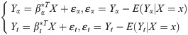
The multiple-to-multiple linear regression model is the basis of the multiple-to-multiple path analysis, so it was introduced firstly. Define the following assumptions: the dependent variable of linear regression is Y = (Y₁,Y₂,⋯,Y_p)^T and the independent variable is X = (X₁,X₂,⋯,X_m)^T. Suppose the joint distribution of $$ \underset{m\times 1}{X}$$ and $$ \underset{p\times 1}{Y}$$ is:

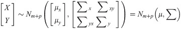
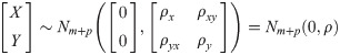
Among them, ρ_x, ρ_xy and ρ_y are the correlation arrays of X,X and Y,Y respectively. ρ is the correlation matrix of [X^T,Y^T]^T. Under the above assumption, the normalized multiple-to-multiple linear regression model is:

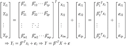
In (3), Y_i = [Y_i1,Y_i2,⋯,Y_ip]^T, x_i = [x_i1,x_i2,⋯,x_im]^T, β* is the regression parameter of the model, i = 1,2,⋯,n. Let n be the number of observations. We assumed that ε~N_p(0,∑_e) is the regression residual and has nothing to do with the value of X.

2.2 Regression hypothesis testing

Path analysis can only be carried out when the standardized regression equation is significant. Therefore, we need to perform the following four types of hypothesis tests for regression analysis before path analysis.

2.2.1 Hypothesis testing of generalized complex correlation coefficient r_xy

In multiple-to-multiple standardized linear regression equations, the joint distribution of X and Y is showed as formula (2), then the generalized determination coefficient is defined as [26]:

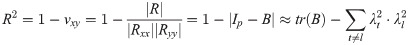
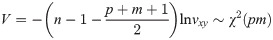
In Eq (4), v_xy is the likelihood ratio statistics for testing independence of X and Y. And $$ R_{xx}={\widehat{\rho }}_x$$, $$ R_{yy}={\widehat{\rho }}_y$$, R in |R| is the correlation matrix of X and Y. $$ B={\displaystyle \sum {}_y^{-1}}{\displaystyle \sum {}_{yx}}{\displaystyle \sum {}_x^{-1}}{\displaystyle \sum {}_{xy}}=R_{yy}^{-1}U$$ is the sample linear correlation matrix of X and Y, U is the regression square sum matrix. $$ {\lambda }_t^2$$ and $$ {\lambda }_l^2$$ are non-zero characteristic roots of B. $$ r_{xy}=R_{\left(x_1{x}_2\cdots x_m\right)\left(y_1{y}_2\cdots y_p\right)}=\sqrt{R^2}$$ is the generalized complex correlation coefficient of X and Y. The invalid assumption of r_xy is H₀:∑_xy = 0.When p>2 and m>2, we can use Bartlett’s approximate chi-square test:

2.2.2 Hypothesis testing of regression equation $$ {\widehat{y}}_{\alpha }=b_{\alpha }^{*T}x\left(\alpha =1,2\cdots ,p\right)$$

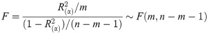
The invalid hypothesis is $$ H_0:{\beta }_{\alpha }^{*}=0$$ and the corresponding F test statistic is:

$$ R_{\left(\alpha \right)}^2$$ is the determination coefficient of X to Y_α

2.2.3 Hypothesis testing of components $$ {\mathit{b}}_{\mathit{j}\mathit{\alpha }}^{*}$$ in $$ {\mathit{b}}_{\mathit{\alpha }}^{*}$$

The invalid hypothesis is $$ H_{0j\alpha }:{\beta }_{j\alpha }^{*}=0$$ and the t test statistic is

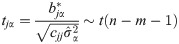
In (7), $$ {\widehat{\sum }}_e=\frac{Q_e}{n-m-1}$$, $$ {\widehat{\sigma }}_{\alpha }^2$$ is the α-th element on the main diagonal of $$ {\widehat{\sum }}_e$$. c_jj is the j-th element on the main diagonal of $$ R_{xx}^{-1}$$.

2.2.4 Hypothesis testing of $$ {\mathit{b}}_{{\mathit{x}}_{\mathit{j}}\mathit{y}}^{*}$$ [27]

The invalid hypothesis is $$ H_0:{({\beta }_{j1}^{*},{\beta }_{j2}^{*},{\beta }_{j3}^{*})}^T=0$$. The F test statistic is:

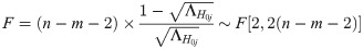
In (8), $$ {\mathrm{\Lambda }}_{H_{0j}}=\frac{\left|Q_e\right|}{\left|Q_{H_{0j}}{}_e\right|}$$. After the above four hypothesis tests, if the standardized multiple linear regression equation is significant, it is meaningful to perform path analysis.

2.3 Path analysis of $$ {\mathit{Y}}_{\mathit{\alpha }}={\mathit{\beta }}_{\mathit{\alpha }}^{*\mathit{T}}\mathit{x}+{\mathit{\epsilon }}_{\mathit{\alpha }}\left(\mathit{\alpha }=\mathbf{1},\mathbf{2},\cdots ,\mathit{p}\right)$$

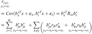
The first step of multiple-to-multiple path analysis is to conduct one-to-multiple path analysis for each dependent variable and all independent variables. According to the established multiple-to-multiple linear regression equation, the path analysis model is performed. The correlation coefficient $$ r_{j{y}_{\alpha }}$$ of each dependent variable Y_α(α = 1,⋯,p) and all independent variables X = (X₁,X₂,⋯,X_m)^T and their determination coefficient $$ R_{\left(\alpha \right)}^2$$ were divided following completely the previous one-to-multiple path analysis model on the basis of standardized linear regression equation [25]. Still further, the decision coefficient was constructed using the existing method [21]. According to the theoretical study of multiple linear regression analysis, the system of regular equations R_xxb* = R_xy about the least squares estimation of β* can be rewritten as:

Fig 1

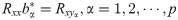
One-to-multiple path analysis diagram.

2.3.1 The division and path of $$ {\mathit{r}}_{\mathit{j}{\mathit{y}}_{\mathit{\alpha }}}$$.

Obviously, the correlation efficient $$ r_{j{y}_{\alpha }}$$ was divided into m terms. There are two types for this m term: $$ b_{j\alpha }^{*}$$ is formed by the path y_α←x_j, so $$ b_{j\alpha }^{*}$$ is called the direct effect of x_j on y_α; and $$ r_{jk}{b}_{k\alpha }^{*}\left(k\ne j\right)$$ is formed by x_j↔x_k→y_α, which is the effect of x_j on y_α through the correlation with x_k and called the indirect effect. Its magnitude can be obtained by multiplying the path coefficients $$ b_{k\alpha }^{*}$$ by the correlation coefficient r_jk, including m-1 items. Finally, $$ r_{j{y}_{\alpha }}$$ is the total effect of x_j on y_α, which is the sum of the direct effect and all the indirect effects.

2.3.2 The division and path of $$ {\mathit{R}}_{\left(\mathit{\alpha }\right)}^{\mathbf{2}}$$.

Among (11): $$ R_{\left(\alpha \right)}^2$$ is the total coefficient of determination of X for Y_α. $$ R_{j\left(\alpha \right)}^{*2}=b_{j\alpha }^{*2}$$ and its corresponding path is y_α←x→y_α. It is called the direct determination coefficient of x_j to y_α.The corresponding path of $$ R_{jk\left(\alpha \right)}^{*}=2b_{j\alpha }^{*}{r}_{jk}{b}_{k\alpha }^{*}$$ is y_α←x_j↔x_k→y_α. It is called the correlation determination coefficient of x_j through the correlation with x_k(k≠j) to y_α.

2.3.3 The decision coefficient R_α(j) and hypothesis test [22]

The comprehensively determine ability of x_j to y_α can be represented by the decision coefficient based on the division of $$ R_{\left(\alpha \right)}^2$$. Its specific expression and hypothesis test are:

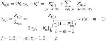
The definition indicates that R_α(j) equals to the sum of the direct determination coefficient $$ R_{j\left(\alpha \right)}^{*2}=b_{j\left(\alpha \right)}^{*2}$$ and the correlation determination coefficient $$ R_{jk\left(\alpha \right)}^{*}=2b_{j\alpha }^{*}{r}_{jk}{b}_{k\alpha }^{*}\left(k\ne j\right)$$. In fact, the decision coefficient is the sum of all determination coefficients related to x_j. The decision coefficient was used to determine the main decision variables and restrictive variables affecting Y_α.

2.4 Multiple-to-multiple path analysis central theorem

The second step is to conduct multiple-to-multiple path analysis. And the innovation is that the correlation between Y caused by the common cause X is considered and three other types of paths are generated. For convenience of observation, let p = 3, m = 3 as an example to make a multiple-to-multiple path analysis diagram as Fig 2. But, the theoretical analysis is based on m independent variables and p dependent variables.

Fig 2

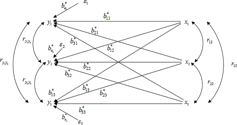
Multiple-to-multiple path analysis diagram.

The multiple-to-multiple path analysis model considered the correlation among different dependent variables compared to the one-to-multiple path analysis model. Accordingly, the central theorem of multiple-to-multiple path analysis is proposed. Based on model (3), for two different Y_α and Y_t, their models are:

In (13), ε_α and ε_t are independent of each other and have nothing to do with the value of X. Since Y_α, Y_t and X have been standardized, the correlation coefficients of Y_α and Y_t, and the corresponding path theoretically is:

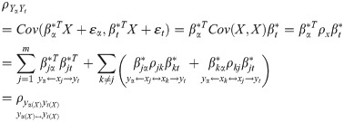
Among them, j = 1,2,⋯,m; k = 1,2,⋯,m; and α = 1,2,⋯,p; t = 1,2,⋯,p. Eq (14) and Eq (15) are called the central theorem of multiple-to-multiple path analysis.

The central theorem demonstrated that $$ {\rho }_{Y_{\alpha }{Y}_t}$$, $$ r_{y_{\alpha }{y}_t}$$ equal to the sum of m² items composite path coefficient. Wherein, the direct path y_α←x_j→y_t has m items. Due to the correlation among independent variables x_j↔x_k(k≠j), the two types of indirect paths were formed as y_α←x_j↔x_k→y_t, y_α←x_k↔x_j→y_t. And x_j↔x_k(k≠j) has $$ C_m^2=\frac{1}{2}m\left(m-1\right)$$ items. So the total composite path number is $$ m+2\times \frac{1}{2}m\left(m-1\right)=m^2$$ items. In addition, the central theorem also showed that three other types of paths generated when the correlation between different dependent variables y_α and y_t was considered, which was caused by the common X. Therefore, there are five types of paths in multiple-to-multiple path analysis, plus the two types of paths in one-to-multiple path analysis.

In fact, the correlation coefficient in the multiple-to-multiple path analysis central theorem is theoretically the regression square sum matrix U in multiple-to-multiple standardized linear regression. Under the least squares estimation, U can be expressed as follows [16]:

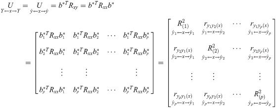
In (16), $$ b_{\alpha }^{*T}{R}_{xx}{b}_t^{*}=r_{{\widehat{y}}_{\alpha }{\widehat{y}}_t\left(x\right)},\alpha \ne t$$ is the correlation coefficient between y_α and y_t caused by the common cause X. Here, U is the determination coefficient matrix of X to Y. $$ R_{\left(\alpha \right)}^2=r_{{\widehat{y}}_{\alpha }{\widehat{y}}_{\alpha }\left(x\right)}^2$$ is the coefficient of determination of X to Y_α. $$ \sqrt{R_{\left(\alpha \right)}^2}=r_{y_{\alpha }\left(x_1{x}_2\cdots x_m\right)}=r_{y_{\alpha }\left(x\right)},\alpha =1,2,\cdots ,p$$ is the complex correlation coefficient of X to Y_α. And in statistics, $$ r_{Y_{\alpha }{Y}_t}$$ is the correlation coefficient of Y_α and Y_t, and has nothing to do with X in the calculation. $$ r_{{\widehat{y}}_{\alpha }{\widehat{y}}_t\left(\alpha \right)}$$ is the determining part of Y_α and Y_t to $$ r_{Y_{\alpha }{Y}_t}$$ due to the common cause X.

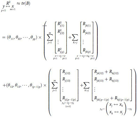
2.5 The division of R²≈tr(B) and its corresponding path

The generalized determination coefficient has been defined using formula (4) before, which was used to reflect the comprehensive determination of all independent variables to all dependent variables [26]. Because the non-zero eigenvalue $$ {\lambda }_t^2\left(t=1,2,\cdots ,k\right)$$ of B is small and $$ 0<{\lambda }_k^2\le {\lambda }_{k-1}^2\le \cdots \le {\lambda }_1^2\le 1$$, the result of $$ {\mathrm{\Sigma }}_{t\ne l}{\lambda }_t^2{\lambda }_l^2$$ is small enough to make R²≈tr(B). In fact, tr(B) is the overestimation of R² here. According to R²≈tr(B), the generalized determination coefficient R² was divided as follows:

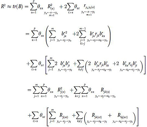
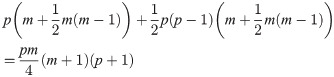
Among (17), θ_αt is the element in matrix $$ R_{{}_{yy}}^{-1}$$. $$ R_{{}_{j(\alpha )}}^2=b_{j\alpha }^{*2}$$ is the direct determination coefficient of x_j on y_α, and the effect path is y_α←x_j→y_α, j = 1,2,⋯,m; α = 1,2,⋯,p. $$ R_{jk\left(\alpha \right)}=2b_{j\alpha }^{*}{r}_{jk}{b}_{k\alpha }^{*}$$ is the indirect determination coefficient of x_j and x_k on y_α, the effect path is y_α←x_j↔x_k→y_α, jk has $$ \frac{1}{2}m\left(m-1\right)$$ items. $$ R_{j\left(\alpha t\right)}=2b_{j\alpha }^{*}{b}_{jt}^{*}$$ is the direct determination coefficient of x_j on y_α and y_t, which is caused by the correlation of y_α and y_t because of the common cause x_j. The effect path is y_α←x_j→y_t, j = 1,2,⋯,m, αt has $$ \frac{1}{2}p\left(p-1\right)$$ items. $$ R_{jk\left(\alpha t\right)}=2b_{j\alpha }^{*}{r}_{jk}{b}_{kt}^{*}$$ is the indirect determination coefficient of x_j and x_k on y_α and y_t. The effect path is y_α←x_j↔x_k→y_t. When α<t, y_α and y_t have $$ \frac{1}{2}p\left(p-1\right)$$ items; when j≠k, jk has $$ \frac{1}{2}m\left(m-1\right)$$ items. $$ R_{kj\left(\alpha t\right)}=2b_{k\alpha }^{*}{r}_{kj}{b}_{jt}^{*}$$ is the indirect determination coefficient of x_j and x_k on y_t and y_α. The effect path is y_α←x_k↔x_j→y_t, when α<t, y_α and y_t have $$ \frac{1}{2}p\left(p-1\right)$$ items; when j≠k, kj has $$ \frac{1}{2}m\left(m-1\right)$$ items. Therefore, the total number of items divided is:

Formula (17) demonstrates that the generalized determination coefficient R² was divided successfully along the five types of paths stated in multiple-to-multiple path analysis central theorem. The specific path vector structure is:

2.6 The generalized decision coefficient R_y(j)

2.6.1 The definition of R_y(j)

In order to describe the comprehensive decision-making ability of x_j to Y, the generalized decision coefficient R_y(j) was defined as follows:

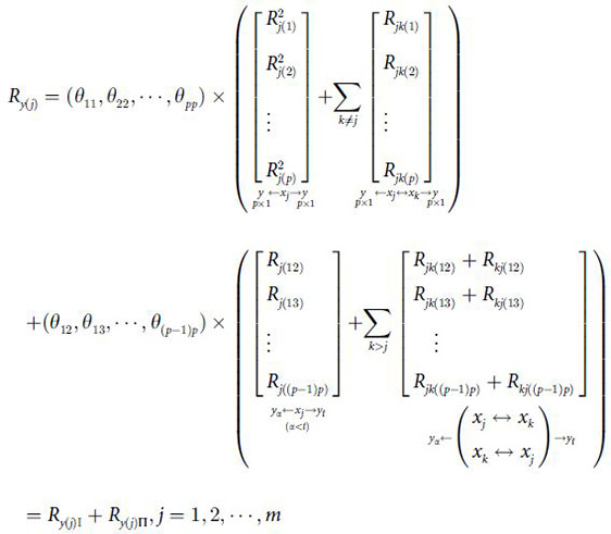
Obviously, the generalized decision coefficient is the sum of the products of $$ R_{j\left(\alpha \right)}^2$$, R_jk(α), R_j(αt) and R_jk(αt)+R_kj(αt) related to x_j in the division and the corresponding elements in $$ R_{yy}^{-1}={\left({\theta }_{\alpha t}\right)}_{p\times p}$$ on the basis of R²≈tr(B). In (19), R_y(j) is divided into two parts: R_y(j)I and R_y(j)II. R_y(j)I is the determination part of x_j and x_j↔x_k to Y_α. R_y(j)Π is the determination part of x_jand x_j↔x_k to Y_α and Y_t(α≠t) due to the common X. In a word, the generalized decision coefficient includes not only the direct determination of x_j to Y_α, Y_α and Y_t(α≠t), but also the indirect determination of x_j↔x_k(k≠j) to Y_α and Y_α and Y_t(α≠t). Specially, the indirect determination considers the correlation among the independent variables and the correlation among the dependent variables at the same time. Therefore, the decision coefficient R_y(j) can be used to express the comprehensive decision ability of x_j to Y.

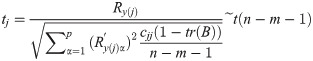
2.6.2 The hypothesis testing of R_y(j)

The invalid hypothesis is H₀:E(R_y(j)) = 0 and the corresponding t test statistic is:

In (20), $$ R_{y\left(j\right)\alpha }^{\text{'}}=\frac{\partial R_{y\left(j\right)}}{\partial b_{j\alpha }^{*}}$$.

3.1 Datasets

In order to demonstrate the effectiveness of the multiple-to-multiple path analysis, the wheat data in arid areas to explore breeding rules was selected to discuss. In detail, the wheat data included thirty-five varieties. These data were obtained in a completely randomized block test, and each sample was set with three repetitions [28]. In multiple-to-multiple path analysis, three indexes closely related to wheat yield was selected as dependent variables: panicles per plant (y₁), grain number per panicle (y₂) and 1000-grain weight (y₃), and three other indexes were selected as independent variables: bio-mass per plant (x₁), single stem grass weight (x₂) and economic coefficient (x₃). Here, economic coefficient refers to the ratio of economic yield to biological yield of wheat.

3.2 Calculation and results

Firstly, the phenotypic correlation matrix of the sample was calculated and expressed as Eq (21). The number of observations for each variable is n = 105.

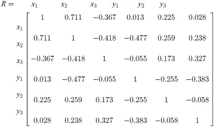
Then, we establish a multiple-to-multiple standardized multiple linear regression equation and calculate the corresponding parameters, the results were written as follow:

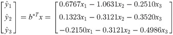
The hypothesis testing of generalized complex correlation coefficient r_xy.

Likelihood ratio statistics of X and Y is v_xy = 0.2987, so χ² = 121.4357**>χ²(3×3), and R² = 1−v_xy = 0.7013, $$ r_{xy}=r_{\left(x_1{x}_2{x}_3\right)\left(y_1{y}_2{y}_3\right)}=\sqrt{R^2}={0.8374}^{**}$$. The results showed that the linear regression of Y to X was extremely significant.

The hypothesis testing of regression equation $$ {\widehat{y}}_{\alpha }=b_{\alpha }^{*T}x\left(\alpha =1,2,3\right)$$.

The values of F test statistics are F₁ = 37.9188**, F₂ = 25.394**, F₃ = 14.408**, respectively. They were all greater than F_0.01(3,101) = 4.007, which showed that each standardized regression equation was extremely significant.

The hypothesis testing of components $$ b_{j\alpha }^{*}$$ in $$ b_{\alpha }^{*}$$

The results of hypothesis testing of components $$ b_{j\alpha }^{*}$$ in $$ b_{\alpha }^{*}$$ were listed in Table 1.

Table 1

t test statistics value of $$ {\mathit{b}}_{\mathit{j}\mathit{\alpha }}^{*}$$.

	y1	y2	y3
x1	6.8994**	1.0212	-1.8092
x2	-105852**	2.3527**	4.9257**
x3	-3.3060**	3.5101**	5.4202**

Among them, except x₁ was not significant to y₂ and y₃, the others were extremely significant.

4The hypothesis testing of $$ b_{x_{j}y}^{*}$$

The results are F₁ = 8.670**, F₂ = 25.394**, F₃ = 10.384**, and the test results were all extremely significant.

Except x₁ is not significant to y₂ and y₃, the above test results showed that the established multiple-to-multiple standardized linear regression equations were extremely significant. The path analysis and decision analysis can be performed subsequently.

Secondly, one-to-multiple path analysis of $$ Y_{\alpha }={\beta }_{\alpha }^{*T}x+{\epsilon }_{\alpha }\left(\alpha =1,2,\cdots ,p\right)$$ was conducted according to the theory before (Method, Part 2.3). The detailed division results of the correlation coefficient and the determination coefficient were listed in Table 2 and Table 3. The decision analysis was also conducted and the results were also listed in Table 3.

Table 2

The division results of the correlation coefficient about $$ {\mathit{Y}}_{\mathit{\alpha }}={\mathit{\beta }}_{\mathit{\alpha }}^{*\mathit{T}}\mathit{x}+{\mathit{\epsilon }}_{\mathit{\alpha }}\left(\mathit{\alpha }=\mathbf{1},\mathbf{2},\mathbf{3}\right)$$.

	xj to yα	Direct effect	xj↔yα	$$	Indirect effect	$$	Total effect
	x1 to y1	0.6767**	x1↔x2→y1	-0.7559	-0.66638(3)	0.2328(1)	0.013(1)
			x1↔x3→y1	0.0921
1	x2 to y1	-1.0631**	x2↔x1→y1	0.4811	0.5860(1)	-0.3115(3)	-0.477(3)
			x2↔x3→y1	0.1049
	x3 to y1	0.251**	x3↔x1→y1	-0.2483	0.1960(2)	0.1970(2)	-0.055(2)
			x3↔x2→y1	0.4444
	x1 to y2	0.1323(3)	x1↔x2→y2	0.2219	0.0927(1)	0.0455(2)	0.225(2)
			x1↔x3→y2	-0.1292
2	x2 to y2	0.3121(2)	x2↔x1→y2	0.0941	-0.0530(2)	0.0914(1)	0.259(1)
			x2↔x3→y2	-0.1471
	x3 to y2	0.3520(1)	x3↔x1→y2	-0.0486	-0.1791(3)	-0.2763(3)	0.173(3)
			x3↔x2→y2	0.1305
	x1 to y3	-0.2150*(3)	x1↔x2→y3	0.4262	0.2432(1)	-0.074(2)	0.028(3)
			x1↔x3→y3	-0.1830
3	x2 to y3	0.5994**(1)	x2↔x1→y3	-0.1529	-0.3613(3)	0.1757(1)	0.238(2)
			x2↔x3→y3	-0.2084
	x3 to y3	0.4986**(2)	x3↔x1→y3	0.0789	-0.1716(2)	-0.3914(3)	0.327(1)
			x3↔x2→y3	-0.2505

Table 3

The division results of determination coefficient $$ {\mathit{Y}}_{\mathit{\alpha }}={\mathit{\beta }}_{\mathit{\alpha }}^{*\mathit{T}}\mathit{x}+{\mathit{\epsilon }}_{\mathit{\alpha }}\left(\mathit{\alpha }=\mathbf{1},\mathbf{2},\mathbf{3}\right)$$.

	yα←xj→yα	Direct determination	yα←xj↔xk→yα	$$	indirect determination	Decision coefficient
	y1←x1→y1	0.4579	y1←x1↔x2→y1	-1.0230	-0.8983	-0.4404**(3)
			y1←x1↔x3→y1	0.1247
1	y1←x2→y1	1.1302	y1←x2↔x1→y1	-1.0230	-1.2461	-0.1159(2)
			y1←x2↔x3→y1	-0.2231
	y1←x3→y1	0.0630	y1←x3↔x1→y1	0.1247	-0.0984	-0.0354(1)
			y1←x3↔x2→y1	-0.2231
	y2←x1→y2	0.0175	y2←x1↔x2→y2	0.0587	0.0245	0.0420*(2)
			y2←x1↔x3→y2	-0.0342
2	y2←x2→y2	0.0974	y2←x2↔x1→y2	0.0587	-0.0331	0.0643**(1)
			y2←x2↔x3→y2	-0.0918
			y2←x3↔x1→y2	-0.0342
	y2←x3→y2	0.1239			-0.1260	-0.0021(3)
			y2←x3↔x2→y2	-0.0918
	y3←x1→y3	0.0462	y3←x1↔x2→y3	-0.1833	-0.1046	-0.0584(2)
			y3←x1↔x3→y3	0.0787
			y3←x2↔x1→y3	-0.1833
3	y3←x2→y3	0.3593			-0.4331	-0.0738(3)
			y3←x2↔x3→y3	-0.2498
			y3←x3↔x1→y3	0.0787
	y3←x3→y3	0.2486			-0.1711	0.0775*(1)
			y3←x3↔x2→y3	-0.2498

The t test statistics values of decision coefficient hypothesis testing were listed in Table 4.

Table 4

t test statistics value of $$ {\mathit{R}}_{\mathit{\alpha }\left(\mathit{j}\right)}^{*}$$.

	y1	y2	y3
x1	-3.39774**	2.3205*	-1.2288
x2	-0.74458	4.5633**	-0.7716
x3	-0.9793	-0.0636	2.4488*

In one-to-multiple path analysis, the results of correlation coefficient division showed that the total effect of biomass per plant (x₁), single stem grass weight (x₂) and economic coefficient (x₃) are all positive and the largest to panicles per plant (y₁), grain number per pancicle (y₂), 1000-grain weight (y₃), respectively. Differently, the direct effect of x₁ to y₁ is the positive and the largest, while the indirect effect is negative and the smallest. The direct effect of x₂ to y₂, x₃ to y₃ are not the largest, but the total effect becomes the largest through the correlation regulation by the indirect effect. The results of the determination coefficients division and the decision coefficients showed that for y₁, x₁ is a very significant restrictive factor; for y₂, x₂ is a very significant positive factor and x₁ is a significant positive factor; for y₃, x₃ is a significant positive factor. These results meant that single stem grass weight (x₂) and economics coefficient (x₃) need to be increased in order to increase grain number per pancicle (y₂) and 1000-grainweight (y₃), but panicles per plant (y₁) will decrease according due to the negative correlation x₂, x₃ and y₁. Meanwhile, biomass per plant (x₁) should be decreased in order to increase the panicles per plant (y₁), but grain number per pancicle (y₂) will decrease here. The contradictory decision-making results of different independent variables (x_i) to different dependent variables (y_i) often lead to the confusion of breeders.

Therefore, after the one-to-multiple path analysis, the multiple-to-multiple path analysis was practiced by taking into account the correlation between the dependent variables. According to formula (17–19), the generalized determination coefficient R² was divided and the results were listed in Table 5.

Table 5

The division results about three other types paths of the generalized determination coefficients.

a	yα←xj→yt	direct determination	yα←xj↔xk→yα	$$
	y1←x1→y2	0.1791	y1←x1↔x2→y2	0.3003
			y1←x1↔x3→y2	-0.1748
1	y1←x2→y2	-0.6636	y1←x2↔x1→y2	-0.2000
			y1←x2↔x3→y2	0.3128
	y1←x3→y2	-0.1767	y1←x3↔x1→y2	0.0244
			y1←x3↔x2→y2	0.0655
	y1←x1→y3	-0.2910	y1←x1↔x2→y3	0.5768
			y1←x1↔x3→y3	-0.2477
2	y1←x2→y3	-1.2744	y1←x2↔x1→y3	0.3253
			y1←x2↔x3→y3	0.4431
	y1←x3→y3	-0.2503	y1←x3↔x1→y3	-0.0396
			y1←x3↔x2→y3	0.1258
	y2←x1→y3	-0.0569	y2←x1↔x2→y3	0.1128
			y2←x1↔x3→y3	-0.0484
3	y2←x2→y3	0.3741	y2←x2↔x1→y3	-0.0955
			y2←x2↔x3→y3	-0.1301
	y2←x3→y3	0.3510	y2←x3↔x1→y3	0.0556
			y2←x3↔x2→y3	-0.1764

The specific calculation of path vector structure is as follows:

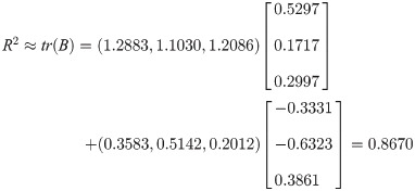
From the previous calculation, we can get tr(B) = 0.8671. The above division of the generalized coefficient of determination is reasonable according to R²≈tr(B). The decision analysis of the model was carried out continually. The decision coefficient of each independent variable to Y = (y₁,y₂,y₃)^T was calculated as follows:

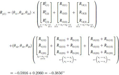
Similar available: R_y(2) = −0.1157, R_y(3) = 0.0906*. According to the decision coefficient, the t test about R_y(j) is further conducted, and the result is t₁ = −4.3943**, t₂ = 0.9293, t₃ = 2.0785**. In addition, it should be noted that the determination coefficients of x_j and x_j↔x_k to y_α have been calculated by one-to-multiple path analysis model (Table 3). The comparison of the results of Table 3 and those of Table 5 demonstrated that great changes have taken place in the regulation of x_j to Y when the correlation among dependent variables was considered. Firstly, the direct and indirect regulations of x_j, x_j↔x_k to Y also were greatly affected by the correlation among Y because of common X. As shown in Table 3, the direct determination of x₂ to y₁, y₂ were both positive, respectively ($$ R_{1\left(2\right)}^2=1.1302y_1\leftarrow x_2\to y_1;R_{2\left(2\right)}^2=0.0974$$ y₂←x₂→y₂). But in Table 5, the direct determination of x₂ to y₁ and y₂ became negative (R₁₂₍₂₎ = -0.6636 y₁←x₂→y₂). This change was due to the consideration of the negative and large correlation of y₁ and y₂ $$ \left(r_{y_1{y}_2}=-0.255\right)$$. Similarly, the direct determination of x₂ to y₂ and y₃ was still changed (R₂₃₍₂₎ = 0.3741 y₂←x₂→y₃), compared to the previous determination coefficient $$ (R_{2\left(2\right)}^2=0.0974y_2\leftarrow x_2\to y_2;R_{3\left(2\right)}^2=0.3593y_3\leftarrow x_2\to y_3)$$. Different from the above, this change was small and both were positive. This phenomenon showed that the small correlation of y₂ and y₃ $$ \left(r_{y_2{y}_3}=-0.058\right)$$ had little influence on the direct determination of x₂ to y₂ and y₃. The direct determination of x₃ to y₂ and y₃ was exactly like the direct determination of x₂ to y₂ and y₃. The indirect determination due to the correlation of x_j↔x_k also changed a lot because of consideration of the correlation among Y. For example, the indirect determination of x₁↔x₂ to y₁and y₃ was 0.5768(y₁←x₁↔x₂→y₃) and 0.3253(y₁←x₂↔x₁→y₃). It’s strange that the original indirect determination of x₁↔x₂to y₁, x₁↔x₂ to y₃ were -1.023 (y₁←x₁↔x₂→y₁) and 0.1833(y₃←x₁↔x₂→y₃), respectively. It is obvious that the strong negative correlation of y₁ and y₃ $$ \left(r_{y_1{y}_3}=-0.383\right)$$ led to the change of indirect regulation. These big changes were enough to show the importance of considering the correlation among Y. There were similar changes in the direct determination of x₁↔x₂ to y₁and y₂(y₁←x₁↔x₂→y₂, y₁←x₂↔x₁→y₂) and x₂↔x₃ to y₁ and y₃(y₁←x₂↔x₃→y₃ y₁←x₃↔x₂→y₃). Secondly, the decision coefficients results showed that x₁ is the very significant restrictive decision factor of Y = (y₁,y₂,y₃)^T (R_y(1) = −0.3856**). But x₁ is the significant positive decision factor to y₂(R_y2(1) = 0.0420*) and is not significant to y₃(R_y3(1) = -0.0584). This phenomena seemed to be caused by the very significant negative decision making effect of x₁ to y₁, and strong negative correlation between y₁ and y₂ $$ \left(r_{y_1{y}_2}=-0.255\right)$$, y₁ and y₃ $$ \left(r_{y_1{y}_3}=-0.383\right)$$. For x₂, there is no point in making a decision. (R_y(2) = −0.1157). And x₃ became a significant positive decision factor to $$ Y={\left(y_1,y_2,y_3\right)}^T\left(R_{y_{\left(3\right)}}=0.0{906}^{*}\right)$$. However, x₃ is significant only to y₃ $$ \left(R_{y_3\left(3\right)}={0.0775}^{*}\right)$$, and is not significant to y₁, y₂ in one-to-multiple path analysis. Obviously, the correlation among Y due to common X makes a big difference in the decision making. The results showed that the economic coefficient (x₃) should be increased, the biomass per plant (x₁) should be appropriately reduced and the single stem grass weight (x₂) should remain unchanged in the process of wheat breeding. These results were in accordance with the existing documents results [28]. In short, the consideration of the correlation among Y caused a big change of the direct determination, the indirect determination and the decision analysis results of x_j to Y. And the greater the correlation among Y is, the greater the impact on regulation.