
Competing Interests: The authors have declared that no competing interests exist.
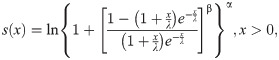
In this study, a new flexible lifetime model called Burr XII moment exponential (BXII-ME) distribution is introduced. We derive some of its mathematical properties including the ordinary moments, conditional moments, reliability measures and characterizations. We employ different estimation methods such as the maximum likelihood, maximum product spacings, least squares, weighted least squares, Cramer-von Mises and Anderson-Darling methods for estimating the model parameters. We perform simulation studies on the basis of the graphical results to see the performance of the above estimators of the BXII-ME distribution. We verify the potentiality of the BXII-ME model via monthly actual taxes revenue and fatigue life applications.
Data analysis is imperious in every aspect of statistical analysis. The statistical characteristics such as skewness, kurtosis, bimodality, monotonic and non-monotonic failure rates are obtained from datasets. The selection of a suitable model for data analysis is a challenging task because it depends on the nature of the dataset. However, if a wrong model is applied to analyze the dataset it leads to loss of information and invalid inferences. It is obligatory to identify the most suitable model for the given dataset.
In the recent decade, many continuous distributions have been introduced in the statistical literature. Some of these distributions, however, are not flexible enough for data sets from survival analysis, life testing, reliability, finance, environmental sciences, biometry, hydrology, ecology and geology. Hence, the applications of the generalized models to these fields are clear requisite. The generalization techniques such as either inserting one or more shape parameters or transforming of the parent distribution are useful to (i) increase the applicability of a parent distribution; (ii) explore skewness and tail properties and (iii) improve the goodness-of-fit of the generalized distributions.
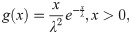
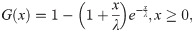
A flexible model for the analysis of lifetime data sets is often attractive to the researchers. The moment exponential (ME) distribution was established by Dara and Ahmad [1]. The probability density function (pdf) and cumulative distribution function (cdf) of the ME distribution are given, respectively, by
The odds ratio for the ME random variable X is given by
During the recent years, the ME distribution has been of great interest in literature. Some new extensions of the ME distribution are: exponentiated ME (EME) distribution (Hasnain et al. [2]), generalized exponentiated ME (GEME) distribution (Iqbal et al. [3]), Weibull ME (WME) distribution (Hashmi et al. [4]) and Topp-Leone moment exponential distribution (Abbas et al. [5]). However, new flexible generalizations of the ME distribution are still needed.
The Burr-XII (BXII) distribution among Burr family (Burr [6]) is widely applied to model insurance data and failure time data. Many generalization of the BXII distributions are available in literature such as Burr XII power series (Silva and Cordeiro [7]), Burr XII modified Weibull (Mdlongwa et al. [8]), Burr XII Uniform (Nasir et al. [9]), Burr XII—Weibull (Kyurkchiev et al. [10]), Burr XII system of densities (Cordeiro et al. [11]), New Burr XII-Weibull-logarithmic (Oluyede et al. [12]), Burr XII-exponential (Yari and Tondpour [13]), Burr XII-Burr XII (Gad et al. [14]) and Burr XII inverse Rayleigh (Goual and Yousof [15]).
The idea here is to incorporate the ME distribution into a larger family through an application of the Burr XII (BXII) distribution. In fact, based on the T-X transform defined by Alzaatreh et al. [16], we construct the BXII-ME distribution.
The study is based on the following motivations: (i) to generate distributions with symmetrical, right-skewed, left-skewed, J, reverse-J and bimodal shaped as well as high kurtosis; (ii) to have monotone and non-monotone failure rate function; (iii) to study numerically the descriptive measures for the BXII-ME distribution based on the parameter values; (iv) to derive mathematical properties such as random number generator, sub-models, ordinary moments, conditional moments, reliability measures and characterizations; (v) to perform the simulation study on the basis of the graphical results to see the performance of maximum likelihood, maximum product spacings, least squares, weighted least squares, Cramer-von Mises and Anderson-Darling estimators; (vi) to reveal the potentiality of the BXII-ME model; (vii) to work as the preeminent substitute model and (viii) to deliver a better fit model than the existing models.
The contents of the article are structured as follows. Section 2 derives the BXII-ME model. We study basic structural properties such as random number generator and sub-models for the BXII-ME model. Section 3 presents certain mathematical properties such as the ordinary moments, conditional moments, reliability measures and characterizations. Section 4 addresses six estimation methods to estimate the BXII-ME parameters. In Section 5, we perform simulation studies on the basis of the graphical results to see the performance of maximum likelihood, maximum product spacings, least squares, weighted least squares, Cramer-von Mises and Anderson-Darling estimators of the BXII-ME distribution. In Section 6, we apply the BXII-ME distribution to two real data sets by adopting maximum likelihood estimation method. We also verify the potentiality of the BXII-ME model. In Section 7, we conclude the article.
In this section, we derive the BXII-ME distribution from the T-X family technique. We also obtain the BXII-ME model by linking the exponential and gamma variables. Basic structural properties are studied. Then, we highlight the nature of the density and failure rate functions.
To obtain a wider family of distributions, Alzaatreh et al. [16] derived the cdf for the T-X family as follows:
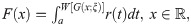
W[G(x; ξ)]∈[a, b],
W[G(x; ξ)] is differentiable and monotonically non-decreasing and
.
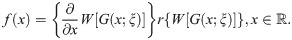
For the T-X family of distributions, the pdf of X is given by
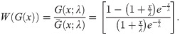
We derive the cdf of the BXII-ME distribution via the T-X family technique by setting

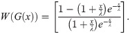
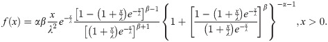
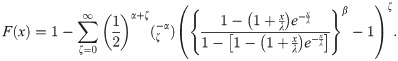
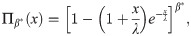
Then, the cdf of BXII-ME distribution is
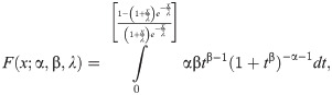
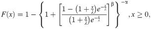
In future, a random variable (rv) with pdf (6) is denoted by X~BXII-ME (α,β,λ). For α = 1, the BXII-ME distribution reduces to the Log-logistic-ME (LL-ME) and for β = 1, the BXII-ME distribution reduces to the Lomax-ME (L-ME).
We derive the BXII-ME distribution from the nexus between exponential and gamma variables.
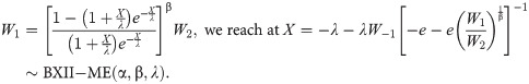
Lemma (i): Let W1 and W2 be independently distributed random variables but have different probability distributions. The random variable W1 has exponential distribution with parameter value 1, i.e. W1~exp(1) and W2 has gamma distribution with parameters α and 1, i.e. W2~gamma (α, 1), then for
Proof
If W1~exp(1), i.e. .
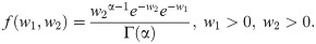
If W2~gamma(α,1), i.e. Then, the joint distribution of two random variables (rvs) is
Letting , the joint density of the rvs X and W2 is
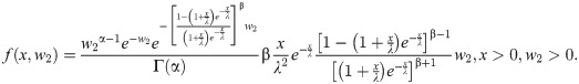
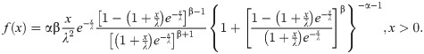
The BXII-ME density of X is
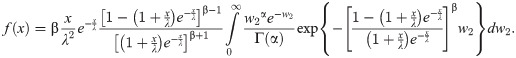
After simplifying, we attain at
Hence the proof is completed.
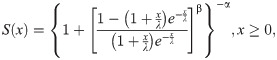
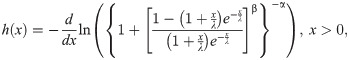
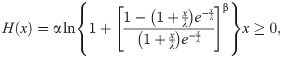
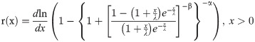
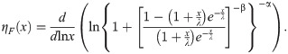
If X~BXII-ME (α,β,λ), the survival, failure rate, cumulative hazard and reverse hazard functions and elasticity of X are given, respectively, by
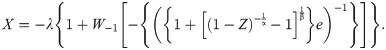
The quantile function of the BXII-ME distribution for 0<q<1 is
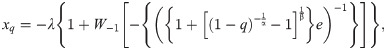
Then, the rv
Since we do not decide shapes of the density and hazard rate functions analytically, we plot them based on some selected parameters values to see their possible shapes. Fig 1 displays that BXII-ME density can take various shapes such as symmetrical, right-skewed, left-skewed, J, reverse-J and bimodal. Fig 2 shows that failure rate function can be modified bathtub, bathtub, inverted bathtub, increasing, decreasing, increasing-decreasing and decreasing-increasing-decreasing shaped. Therefore, the BXII-ME distribution is quite flexible and can be applied to numerous data sets.

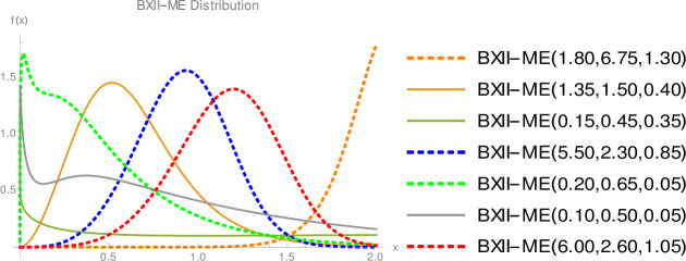
Plots of the BXII-ME density.
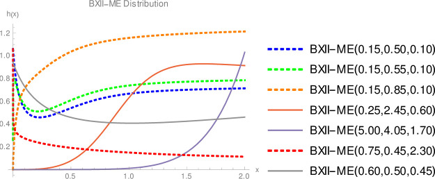
Plots of the BXII-ME hazard rate.
In this subsection, we provide a useful linear representation for the density of X, which can be used to derive some mathematical properties of the BXII-ME model. The cdf (5) can be expressed as
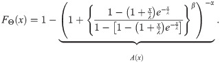
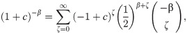
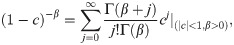
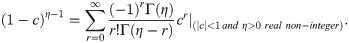
First, we shall consider the three power series
Applying (15) for A(x) in (14), we obtain
Second, using the binomial expansion, the last equation can be expressed as
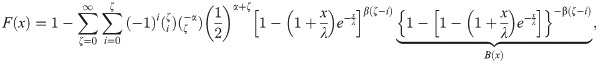
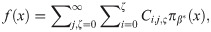
Third, applying (16) for B(x) in the last equation, we can write
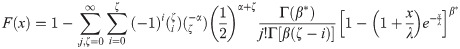
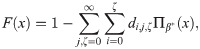
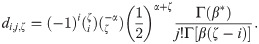
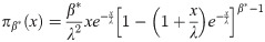
Upon differentiating (18), we obtain

We present some of its mathematical properties such as the ordinary moments, the Mellin transform, conditional moments, reliability measures and characterization in this segment.
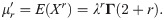
The moments are significant tools for statistical analysis in pragmatic sciences. The rth moment about the origin is

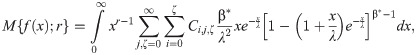
The Mellin transformation is applied to obtain the moments as

The rth central moment (μr), skewness (γ1) and kurtosis (γ2) for the BXII-ME model are obtained from and .The numerical values for mean , median , dispersion (σ), γ1 and γ2 for the BXII-ME distribution for selected values of α,β,λ are listed in Table 1.

| α,β,λ | σ | γ1 | γ2 | ||
|---|---|---|---|---|---|
| 0.5,0.5,0.5 | 2.6776 | 1.9401 | 8.6517 | 74.8778 | 6089.09 |
| 1,0.5,0.5 | 1.3043 | 0.8388 | 1.3588 | 1.6362 | 6.3791 |
| 2,0.5,0.5 | 0.6059 | 0.3354 | 0.7108 | 2.0698 | 8.5074 |
| 3,0.5,0.5 | 0.3737 | 0.2033 | 0.4608 | 2.4150 | 10.7472 |
| 4,0.5,0.5 | 0.2611 | 0.1442 | 0.3276 | 2.7008 | 13.4562 |
| 5,0.5,0.5 | 0.1983 | 0.1119 | 0.2486 | 2.8423 | 14.8636 |
| 0.5,1,0.5 | 1.6534 | 1.3440 | 1.2528 | 1.5988 | 7.3620 |
| 0.5,2,0.5 | 1.2092 | 1.0763 | 0.6183 | 1.5854 | 7.3019 |
| 0.5,3,0.5 | 1.0717 | 0.9936 | 0.4024 | 1.5638 | 7.6506 |
| 0.5,4,0.5 | 1.0064 | 0.9534 | 0.2950 | 1.5012 | 7.5854 |
| 0.5,5,0.5 | 0.9690 | 0.9298 | 0.2314 | 1.4358 | 7.3989 |
| 0.5,0.5,1 | 5.1601 | 3.8796 | 4.8952 | 1.5752 | 6.7218 |
| 0.5,0.5,2 | 10.3192 | 7.7575 | 9.7881 | 1.5745 | 6.7248 |
| 0.5,0.5,3 | 15.4789 | 11.6344 | 14.6839 | 1.5752 | 6.7266 |
| 0.5,0.5,4 | 20.6384 | 15.5133 | 19.5786 | 1.5746 | 6.7190 |
| 0.5,0.5,5 | 25.7992 | 19.3969 | 24.4738 | 1.5746 | 6.7197 |
| 1.7,5,0.65 | 1.0197 | 1.0212 | 0.1502 | 0.0016 | 3.6538 |
| 2,5,0.65 | 0.9984 | 1.0021 | 0.1426 | -0.1139 | 3.5415 |
| 5,2.85,0.5 | 0.5972 | 0.6019 | 0.1350 | -0.1462 | 3.0058 |
| 5,2.8,0.5 | 0.5938 | 0.5982 | 0.1366 | -0.1322 | 2.9973 |
| 5,2,0.5 | 0.5219 | 0.5190 | 0.1660 | 0.1593 | 2.9411 |
| 5.5,1.7398,0.5 | 0.4735 | 0.4664 | 0.1712 | 0.2921 | 3.0000 |
Life expectancy, mean waiting time and inequality measures can be obtained from the incomplete moments.
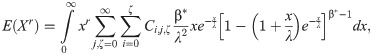
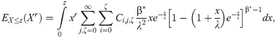
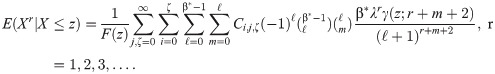
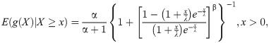
The rth conditional moment E(Xr|X>z) is The rth lower incomplete moment EX≤z(Xr) is
The rth conditional moment is

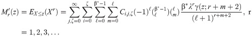
The rth reversed conditional moment E(Xr|X≤z) for X~BXII-ME (α,β,λ), is
The mean deviation about the mean (δ1 = E|X−μ|) and about the median can be written as and , respectively, where μ = E(X) and . The quantities and can be obtained from (22). For specific probability p, Lorenz and Bonferroni curves are computed as and B(p) = L(p)|p, where q = Q(p).
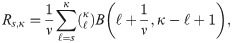
Consider a system with κ identical elements, out of which s elements are operative. Let Xi,i = 1,2…κ represent the strengths of κ elements with the cdf F while, the stress Y enforced on the elements has the cdf G. The strengths Xi and stress Y are independently and identically distributed (i.i.d.). The probability that system operates properly, is the reliability of the system, i.e.

Then, we can write this probability (from Bhattacharyya and Johnson [18]) as follows:
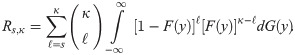
Let X~BXII-ME (α1,β,λ), Y~ BXII-ME (α2,β,λ) with unknown α1 and α2, common β,λ where X and Y are independently distributed. The reliability in multicomponent stress-strength model for the BXII-ME distribution is

Letting , we obtain
Let uv = w, we have
Here, we characterize the BXII-ME distribution via relationship between truncated moments of a function of X with another function. This characterization is stable in the sense of weak convergence (Glänzel [20]).
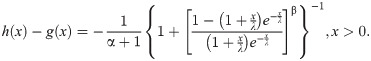
Proposition 3.4.1: Let X:Ω→(0,∞) be a continuous random variable and let
The pdf of X is (6) if and only if the function h(x), in Theorem G (Glänzel [8]), has the form .
Proof If X has pdf (6), then or
Conversely, if h(x) is given as above, then (for x>0)
In view of Theorem G, X has density (6).
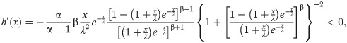
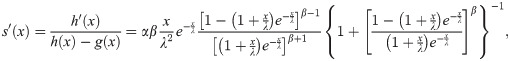
Let X:Ω→(0,∞) be a continuous random variable. The pdf of X is (6) if and only if there exist functions h(x) and g(x) (defined in Theorem G) satisfying the differential equation
The general solution of the differential equation in Corollary 3.4.1 is

In this section, we propose various estimators for estimating the unknown parameters of the BXII-ME distribution. We discuss maximum likelihood, maximum product spacings, least squares, weighted least squares, Cramer-von Mises and Anderson-Darling estimation methods and compare their performances on the basis of simulated sample from the BXII-ME distribution. The details are the followings.
We address parameters estimation using maximum likelihood method. The log-likelihood function for the vector of parameters ξ = (α,β,λ) of the BXII-ME distribution is
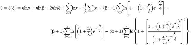
We can compute the maximum likelihood estimators (MLEs) of α,β and λ by solving equations , and .
The maximum product spacing (MPS) method is alternative method for MLE for parameter estimation. This method was proposed by Cheng and Amin [21,22] as well as it was also independently developed by Ranneby [23] as approximation to the Kullback-Leibler measure of information. This method is based on an idea that differences (spacings) between the values of the cdf at consecutive data points should be identically distributed. Let X(1),X(2),…,X(n) be ordered sample of size n from BXII-ME distribution. The geometric mean of the differences is given as
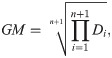
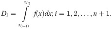
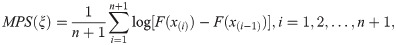
The maximum product spacing (MPS) estimates, say and , of α,β and λ are obtained by maximizing the geometric mean of the differences. Substituting cdf of BXII-ME distribution in Eq (27) and taking logarithm of the above expression, we have
Let X(1),X(2),…,X(n) be ordered sample of size n from BXII-ME distribution. Then, the expectation of the empirical cumulative distribution function is defined as
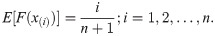
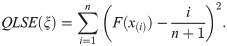
The least square estimates (LSEs) say, and of α,β and λ are obtained by minimizing
Let X(1),X(2),…,X(n) be ordered sample of size n from BXII-ME distribution. The variance of the empirical cumulative distribution function is defined as
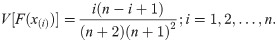
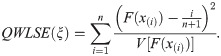
Then, the weighted least square estimates (WLSEs) say, and of α,β and λ are obtained by minimizing
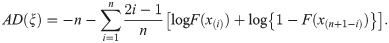
This estimator is based on Anderson-Darling goodness-of-fits statistics which was introduced by Anderson and Darling [24]. The Anderson-Darling (AD) minimum distance estimates, and of α,β and λ are obtained by minimizing
The Cramer-von Mises (CVM) minimum distance estimates, and , of α,β and λ are obtained by minimizing
We refer the interested readers to Chen and Balakrishnan [25] for AD and CVM goodness-of-fits statistics. To solve the above equations, Eqs (26) and (28)–(32) can be optimized either directly by using the R (optim and maxLik functions), SAS (PROC NLMIXED) and Ox package (sub-routine Max BFGS) or employing non-linear optimization tactics such as the quasi-Newton procedure to numerically optimize , MPS(ξ), QLSE(ξ), QWLSE(ξ), AD(ξ) and CVM(ξ) functions.
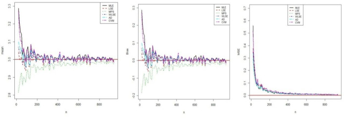
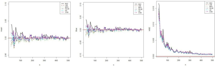
In this Section, we perform the simulation studies by using the BXII-ME to see the performance of the above estimators corresponding to this distribution and obtain the graphical results. We generate N = 1000 samples of size n = 20, 25,…, 500 from BXII-ME distribution with true parameter values α = 0.25,β = 3 and λ = 3. The random numbers generation is obtained by its quantile function. In this simulation study, we calculate the empirical mean, bias and mean square errors (MSEs) of all estimators to compare in terms of their biases and MSEs with varying sample size. The empirical bias and MSE are calculated by (for h = α,β,λ)
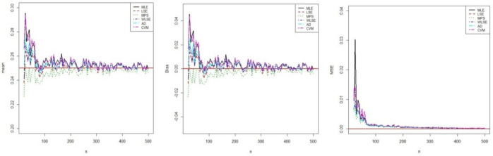
Simulation results of α.
Simulation results of β.
Simulation results of λ.
We verify the potentiality of the BXII-ME model via monthly actual taxes revenue and fatigue life data sets. The first data set represents monthly actual taxes revenue (in 1000 million Egyptian pounds) from January 2006 to November 2010. It is studied by Nassar and Nada [26] and Yousof et al. [27]. The first data set is available at https://doi.org/10.1080/03610918.2017.1377241. The second data set is about the fatigue life of 6061-T6 aluminum coupons cut parallel with the direction of rolling and oscillated at 18 cycles per second (Birnbaum and Saunders [28] and El-Morshedy et al. [29]). The second data set is available at https://doi.org/10.2307/3212004. We compare the BXII-ME distribution with competing models such as Burr III-moment exponential (BIII-ME), Weibull-moment exponential (W-ME), generalized exponentiated moment exponential (GEME), generalized moment exponential (GME), exponentiated moment exponential (EME), moment exponential (ME) and BXII distributions. For the selection of the best fit distribution, we compute the estimate of likelihood ratio statistics (), Akaike information criterion (AIC), corrected Akaike information criterion (CAIC), Bayesian information criterion (BIC), Hannan-Quinn information criterion (HQIC), Cramer-von Mises (W*), Anderson Darling (A*), and Kolmogorov-Smirnov [K-S] statistics with p-values for all competing models. We compute the MLEs and their standard errors (SEs) in parentheses. Chen and Balakrishnan [25] described in detail about the statistics W* and A*. Chen et al. [30] also studied , AIC and BIC. We also compute the MLEs along with their standard errors (SEs) in parentheses. Table 2 reports some descriptive measures for two real data sets.
| N | Min | Max | Mean | Median | Standard deviation | Skewness | Kurtosis | |
|---|---|---|---|---|---|---|---|---|
| Monthly Actual Taxes revenue | 59 | 4.1 | 39.2 | 13.4881 | 10.6 | 8.0515 | 1.6083 | 5.2560 |
| Fatigue Life | 101 | 70 | 212 | 133.7327 | 133 | 22.35571 | 0.3305 | 4.05284 |
Table 2 shows that the monthly actual taxes revenue data set is significantly right-skewed, with significantly positive kurtosis. About the fatigue life data set, it is a right-skewed, with high positive kurtosis.
The boxplots in Fig 6 suggests that both data sets are right-skewed. The nature of the two data sets differs in numerous features. Some extreme points are also present in these data sets.
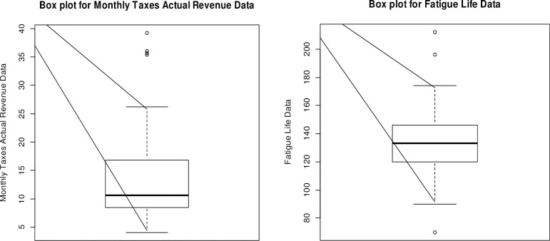
Boxplots of the monthly actual taxes revenue (left) and Fatigue Life (right).
Here, we study the statistical analysis by total time on test (TTT) for the two data sets in Fig 7.
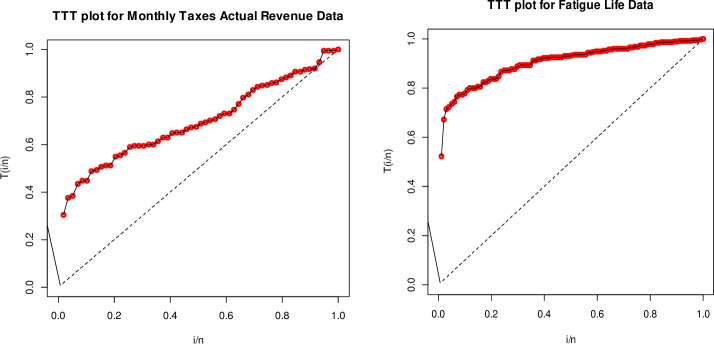
TTT plots of the monthly actual taxes revenue (left) and fatigue life (right).
The TTT plots in Fig 7 for both data sets are concave which suggests increasing failure intensity. So, the BXII-ME distribution is suitable to model these data sets.
Table 3 reports the MLEs, SEs and measures W*, A*, K-S (p-values). Table 4 displays the values of measures , AIC, CAIC, BIC and HQIC.
| Model | α | β | λ | W* | A* | K-S (p-value) |
|---|---|---|---|---|---|---|
| BXII-ME | 0.1601 (0.0724) | 3.4311 (1.0493) | 3.8680 (0.4363) | 0.0304 | 0.2134 | 0.0575 (0.9899) |
| BIII-ME | 1.8961 (0.8784) | 1.1364 (0.2599) | 5.2090 (1.3601) | 0.1606 | 0.9766 | 0.1206 (0.3572) |
| W-ME | 31.4145 (60.7167) | 0.9787 (0.0961) | 58.3359 (63.6252) | 0.2787 | 1.7754 | 0.1409 (0.1918) |
| GEME | 160.3036 (341.4872) | 0.3430 (0.1233) | 0.3016 (0.1854) | 0.05225 | 0.3049 | 0.0637 (0.9702) |
| EME | 2.3384 (0.5638) | --- | 4.5651 (0.5554) | 0.1659 | 1.01409 | 0.1251 (0.3146) |
| GME | --- | 1.3023 (0.1188) | 15.7102 (5.5018) | 0.2288 | 1.4390 | 0.1346 (0.2351) |
| ME | --- | --- | 6.7441 (0.6208) | 0.1949 | 1.2113 | 0.1675 (0.07304) |
| BXII | 0.0669 (0.2672) | 6.08052 (24.2926) | --- | 0.05601 | 0.3254 | 0.4674 (1.269e-11) |
| Model | AIC | CAIC | BIC | HQIC | |
| BXII-ME | 375.2900 | 381.2900 | 381.7264 | 387.5227 | 383.7230 |
| BIII-ME | 383.7592 | 389.7593 | 390.1956 | 395.9919 | 392.1922 |
| W-ME | 393.4770 | 399.4769 | 399.9133 | 405.7096 | 401.9099 |
| GEME | 376.6902 | 382.6901 | 383.1265 | 388.9228 | 385.1231 |
| EME | 384.0488 | 388.0488 | 388.2630 | 392.2038 | 389.6707 |
| GME | 389.1094 | 393.1094 | 393.3237 | 397.2645 | 394.7314 |
| ME | 396.1928 | 398.1928 | 398.2629 | 400.2703 | 399.0038 |
| BXII | 514.4602 | 518.4602 | 518.6745 | 522.6153 | 520.0822 |
From the Tables 3 and 4, it is clear that our proposed model is the best fitted, with the smallest values for all statistics and maximum p-value. Fig 8 suggests that the proposed model is closely fitted to monthly actual taxes revenue.
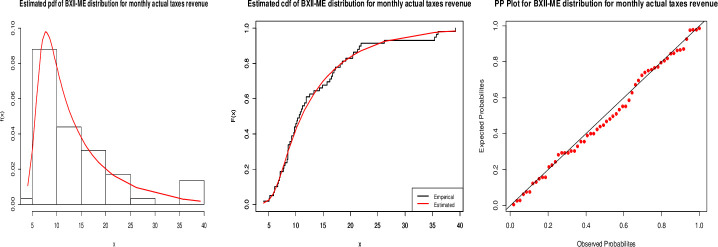
Fitted pdf (left), cdf (center) and PP(right) plots for the BXII-ME distribution to monthly actual taxes revenue.
Table 5 reports the MLEs, SEs (in parentheses) and measures W*, A*, K-S (p-values). Table 6 displays the values of measures , AIC, CAIC, BIC and HQIC.
| Model | α | β | λ | W* | A* | K-S (p-value) |
|---|---|---|---|---|---|---|
| BXII-ME | 1.2646 (0.5203) | 4.7614 (0.6304) | 81.8650 (5.1685) | 0.0368 | 0.2454 | 0.0524 (0.9441) |
| W-ME | 52.5287 (90.9450) | 3.2035 (0.2283) | 160.4654 (43.7269) | 0.1521 | 0.9923 | 0.1013 (0.2512) |
| EME | 91.2087 (31.4517) | --- | 18.8163 (1.2031) | 0.1836 | 1.0314 | 0.1055 (0.211) |
| GEME | 35.3444 (19.9402) | 1.2562 (0.1588) | 77.9056 (68.0432) | 0.1476 | 0.8293 | 0.1009 (0.2557) |
| GME | --- | 2.9483 (0.0141) | 985384.46113 (8451.613) | 0.0571 | 0.3804 | 0.1597 (0.01156) |
| EME | --- | --- | 66.86634 (4.7047) | 0.0625 | 0.3795 | 0.4006 (1.665e-14) |
| BXII | 0.0813 (0.2435) | 2.5205 (7.5487) | --- | 0.0985 | 0.5657 | 0.5923 (< 2.2e-16) |
| Model | AIC | CAIC | BIC | HQIC | |
|---|---|---|---|---|---|
| BXII-ME | 455.128 | 916.2559 | 916.5034 | 924.1013 | 919.432 |
| W-ME | 463.0179 | 932.0358 | 932.2832 | 939.8812 | 935.2118 |
| EME | 461.6561 | 927.3123 | 927.4347 | 932.5425 | 929.4296 |
| GEME | 459.7397 | 925.4793 | 925.7267 | 933.3247 | 928.6554 |
| GME | 469.9547 | 943.9095 | 944.0319 | 949.1397 | 946.0268 |
| EME | 557.8864 | 1117.773 | 1117.813 | 1120.388 | 1118.832 |
| BXII | 754.1948 | 1512.390 | 1512.512 | 1517.620 | 1514.507 |
From the Tables 5 and 6, it is clear that our proposed model is the best fitted, with the smallest values for all statistics and maximum p-value. Fig 9 infers that the proposed model is closely fitted to fatigue life data.
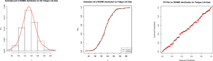
Fitted (left) pdf, (center) cdf and (right) PP plots for the BXII-ME distribution to fatigue life.
We construct the BXII-ME distribution from the T-X family technique. The BXII-ME density highlights various shapes as symmetrical, right-skewed, J, reverse-J, left-skewed, arc and exponential shapes. The BXII-ME failure rate has shapes such as an upside-down bathtub, modified bathtub, constant, increasing, decreasing and increasing-decreasing. We study some of its mathematical properties such as random number generator, sub-models, ordinary moments, conditional moments, reliability measures and characterizations. We employ different estimation methods to estimate the model parameters. We perform simulation studies on the basis of the graphical results to see the performances of the estimators of the BXII-ME distribution. We apply the BXII-ME distribution to two real data sets by adopting maximum likelihood estimation method. The potentiality of the BXII-ME model illustrates that it is flexible, competitive and parsimonious. Therefore it should be included in the distribution theory to facilitate the researchers. Further, as perspective of future projects, we may study some rigorous issues (i) Burr XII generalized moment exponential (BXII-GME) (ii) Burr XII exponentiated moment exponential (BXII- EME); (iii) exponentiated BXII-ME; (iv) unit BXII-ME; (v) bivariate extension of BXII-ME and (vi) discrete case of Burr XII-ME distribution. Future works also includes study of the complexity of the BXII-ME distribution via Bayesian methods. In Bayesian inference, researchers can consider the deviance information criterion (DIC). In this regard, we refer to the articles of [30–35]. We also leave the study of DIC as future work.
Theorem G. Let (Ω,F,P) be a given probability space and let H = [a1,a2] be an interval with a1<a2 (a1 = −∞,a2 = ∞). Let X:Ω→[a1,a2] be a continuous random variable with distribution function F and Let g(x) be a real function defined on H = [a1,a2] such that E[g(X)|X≥x] = h(x) for x∈H is defined with some real function h(x) should be in simple form. Assume that g(x)εC([a1,a2]), h(x)εC2([a1,a2]) and F is twofold continuously differentiable and strictly monotone function on the set [a1,a2].We conclude, assuming that the equation g(x) = h(x) has no real solution in the inside of [a1,a2].Then F is obtained from the functions g(x) and h(x) as , where s(t) is the solution of equation and k is a constant, chosen to make
1
2
3
4
5
6
7
8
9
10
11
12
13
14
15
16
17
18
19
20
21
22
23
24
25
26
27
28
29
30
31
32
33
34
35
 On the Burr XII-moment exponential distribution
 Facebook
 Twitter
 Linkedin
 Whatsapp

