
Competing Interests: The authors have declared that no competing interests exist.
‡ These authors also contributed equally to this work.
Differential equations are commonly used to model various types of real life applications. The complexity of these models may often hinder the ability to acquire an analytical solution. To overcome this drawback, numerical methods were introduced to approximate the solutions. Initially when developing a numerical algorithm, researchers focused on the key aspect which is accuracy of the method. As numerical methods becomes more and more robust, accuracy alone is not sufficient hence begins the pursuit of efficiency which warrants the need for reducing computational cost. The current research proposes a numerical algorithm for solving initial value higher order ordinary differential equations (ODEs). The proposed algorithm is derived as a three point block multistep method, developed in an Adams type formulae (3PBCS) and will be used to solve various types of ODEs and systems of ODEs. Type of ODEs that are selected varies from linear to nonlinear, artificial and real life problems. Results will illustrate the accuracy and efficiency of the proposed three point block method. Order, stability and convergence of the method are also presented in the study.
The multistep method was discovered by Bashforth and Adams [1] in their pursue to extend Euler’s method. The idea which was then named the Adams-Bashforth method was formulated by obtaining the approximated solution for a point by way of solution values from multiple previous steps. Milne [2, 3] then established a new form of multistep method, known as the predictor-corrector formulation. The modern multistep method was widely researched by authors such as [4–9].
Krogh [6], managed to revitalize the field of numerical method for solving ordinary differential equations (ODEs) which was almost discarded as robust, with a divided difference approach. The premise of his work is that the back values of any point of the derivative could be interpolated. In the same study, Krogh presented a comparison for two second order problems similar to the problem provide in [5], where Gear had introduced a Nordsieck version of the multi step method.
The current study is part of research series motivated by [9]. Suleiman [9] developed an algorithm for solving stiff and non stiff higher order ordinary differential equations. The nonstiff portion of the algorithm was derived in a divided difference formulation whereas the stiff algorithm was red obtained using a backward differentiation formulation. Suleiman [9] introduced a divided difference formulation known as Direct Integration (DI) method for solving nonstiff higher order ODEs directly. Omar [10] then established a new variation of the DI method by implementing a block algorithm. The block DI method developed by Omar consists of two different red algorithms, namely explicit block method and implicit block method algorithms. The block method developed in Omar [10] was matched by a fully implicit block method established by Abdul Majid [11]. In [12], authors presented a predictor-corrector algorithm in backward difference form for solving higher ODEs. The backward difference formulation from [12] was then extended in [13]. Md Ijam [13] fitted the backward difference formulae with a two point block algorithm, reducing the number of function evaluations by half.
The current study is established to overcome drawbacks of the DI method as well to provide an efficient numerical multistep method. When establishing a numerical method, accuracy has constantly been the benchmark to determine its viability. But, as numerical methods become more and more robust, accuracy alone is longer sufficient hence, the need for efficiency. The efficiency of a numerical method is associated with computational cost which translates into accuracy per step. The current study proposes a three-point block multistep formulation (3PBCS) in backward difference form for solving higher order ODEs directly. The three-point formulation requires only a fraction of computational steps usually required by standard methods. Complemented with an Adams equivalent predictor-corrector algorithm, the 3PBCS method is able to reduce computational cost more significantly. The drawback of the 3PBCS method, is the need for establishing three set of coefficients for each blocks but, by establishing multiple recursive relationships between explicit and implicit coefficients and also for coefficients of different orders, the corrector algorithm can be written in terms of the predictor which eliminates redundancy in the form of unnecessary calculations. This issue becomes irrelevant if introduced with a parallel algorithm.
Recent advancement in related area can be found in works such as [14–27] and others.
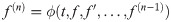
Ordinary differential equations are often used to model the occurrence of natural phenomenon to man made mechanics. Among these applications include modeling two body motions, chemical reactions and engineering problems such as the bend of a thin clamped beam. These ODE models can be categorized into stiff and nonstiff. However, the study conducted here focuses mainly on initial value nonstiff ODEs of any order. We begin by considering the higher order ODE,

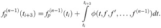
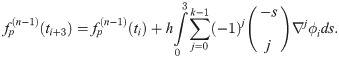
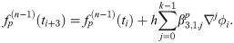
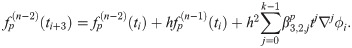
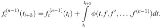
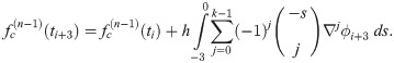
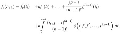
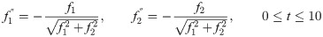
The third point predictor is derived by integrating (1) once with the limit of integration from ti to ti+3 which is then denoted as
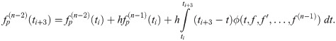
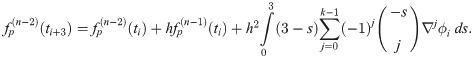
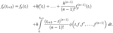

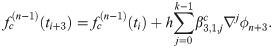
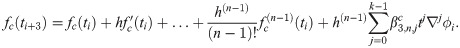
Derivation of the corrector also begins with integrating (1) once, which introduces the corrector as follows
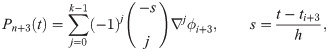
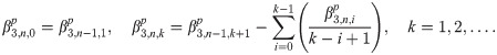
In a three point block predictor-corrector method, it is highly beneficial to obtain the relationship between integration coefficients. In this section, firstly the explicit and implicit integration coefficients are derived. Then a recursive relationship between explicit and implicit integration coefficients and also coefficient of different orders are established.
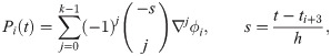
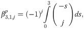
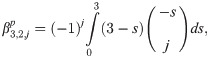
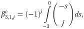
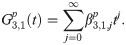
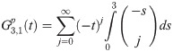
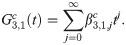
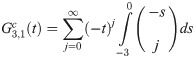
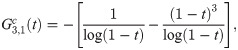
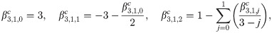
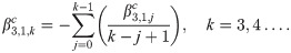
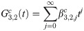
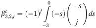
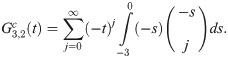
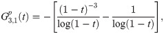
To derive the explicit integration coefficient, we first denote the first order generating function, as

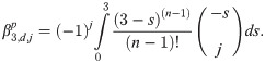
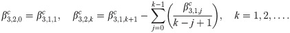
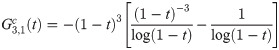
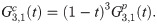
The implicit integration is derived by first defining the first order implicit generating function
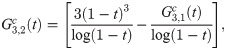
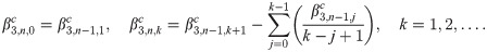
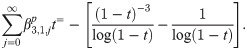
Calculating both predictor and corrector can be expensive, especially when the calculation requires large number of integration. By obtaining a recursive relationship between explicit and implicit coefficients, the corrector can be written in terms of predictor which will reduce the need for extensive calculation to obtain the corrected value. We begin by establishing the recursive interrelationship between explicit and implicit coefficients of the first order. From (13) and (18), the first order explicit and implicit generating functions are given respectively as


Conditions that satisfy order and zero stability of block methods have been researched by authors such as [29–31]. Order and stability of the proposed method presented in this study uses techniques provided in [30]. Before establishing order and stability of the method, here are preliminary definitions that are required.
This section provides necessary definitions to determine issue of stability, convergence and order of the method. We begin with the definition of the general linear multistep method.
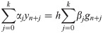
Definition 1 The general linear multistep method is denoted by
Definition 2 The linear differential operator L associated with the linear multistep method is defined
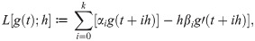
Let g(t) be a function that is q times differentiable. Next, expand g(t + ih) and g′(t + ih) about t and arrange as

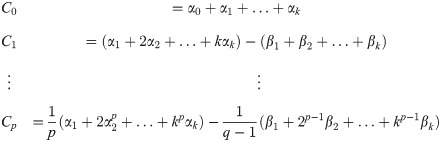
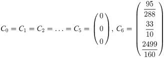
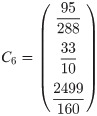
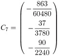
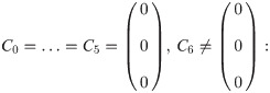
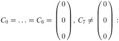
Definition 3 The linear multistep method and associated difference operator L are said to be of order p if, C0 = C1 = … = Cq = 0, Cq+1 ≠ 0 where
Definition 5 A Linear Multistep Method is said to be consistent if the LLM is of order p ≥ 1.
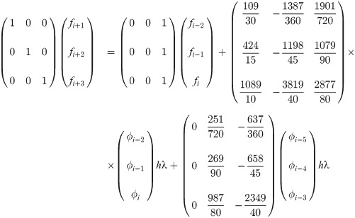
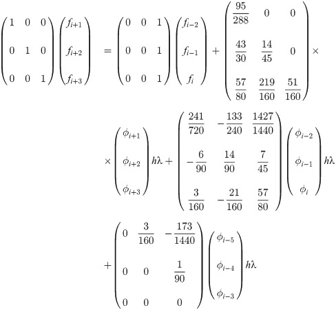
In the current section, order of both predictor and corrector will be substantiated for k = 6 number of back values. For simplicity, the example selected is of f′. Beginning with the predictor, fi+b for b = 1, 2, 3 of the three block method can be expressed as


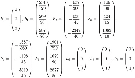
By way of Definition 3, from the set of vector columns yield


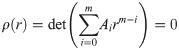
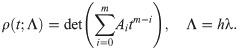
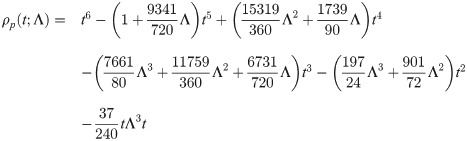
Zero stability governs certain conditions which dictates the viability of a linear multistep method. The stability of the three point block method can be established by following similar conditions as presented in [7]. To establish whether the method is zero stable, derivation begins with the predictor. By way of the standard linear test problem

Works of [32] highlights that certain conditions are required in order to validate the convergence of a backward difference formulation. Those conditions are governed by the following.
Theorem 1 Conditions necessary for the linear multistep method (6) and (10) to be convergent are
Methods must be consistent
Methods must be zero stable
For proof of the theorem, we refer readers to works of [32].
The order of the method was established in earlier subsection as following: The predictor
Finally, we proceed with the subsequent section, the long awaited numerical results.
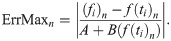
Real life science and engineering problems are often modeled in the form of ODEs. Every so often, these problems are not able to be solved analytically, thus requires numerical approximations. These numerical approximations are often used as alternative solutions due to the absence of analytical solution. The current section provides results for selected higher order ODEs using the proposed three point block method (3PBCS) with constant step size. Problems selected varies from linear to nonlinear artificial and real life problems which are in the form of single and systems of equations. The problems selected also consist of various difficulty levels in order to provide a holistic overview of the 3PBCS method’s capability. For a more just comparison, the 3PBCS method is compared against Direct Integration (DI), one point block (1PBCS) and two point block (2PBCS) methods. Results will be compared in terms of accuracy, function evaluations and efficiency. The error solution used in this study adopts techniques suggested in [12] which is given by
This section begins with higher order differential problems which are artificial in nature and of different orders then followed with well known differential equations. Examples 1-3 are 4th to 5th order problems obtained from various sources.
Example 1: A non homogeneous 4th order ODE,

Example 2: A 4th order non linear ODE
Example 3: A 5th order non linear ODE

Table 1 presents numerical results of the 1PBCS, 2PBCS and 3PBCS methods for Examples 1 -3. The 1PBCS approximates single steps of equidistant, the 2PBCS approximates two-points of equidistant simultaneously and the 3PBCS approximates three-points of equidistant simultaneously. Results will compare accuracy and total steps approximated by all three methods for step sizes 10−1, 10−2, 10−3, 10−4 and 10−5. Tstep represents the total steps required and Err denotes the maximum error estimated for each method in the interval T0 ≤ t ≤ Tn. The 1PBCS and 2PBCS methods were selected to compare efficiency of the 3PBCS when solving higher order ODEs with other backward difference methods to provide a fair analysis. The analysis of Examples 1 to 3 begins with results provided in Table 1. As shown in Table 1, the 3PBCS method obviously requires less calculation steps compared to the latter even though some loss of accuracy is expected. For Example 2, the 3PBCS is able to match the level of accuracy of 1PBCS and 2PBCS methods but slightly under-performed in Examples 1 and 3. Whereas Table 2 provides computational time (Time) which is recorded in seconds for Examples 1-3. As exhibited in Table 2, 3PBCS requires less computational time compared to 1PBCS and 2PBCS methods for almost all step sizes, except at H = 1 × 10⁻¹. This is due to the initial calculation of the three-point block integration coefficients. The small amount of Tsteps required to calculate the solutions from beginning to end outweighs the efficiency of the 3PBCS method. But as a smaller H is selected, more Tstep is required which redistributes calculation time of the initial 3PBCS integration coefficients thus leads to a lesser overall computational time. This loss is barely significant and can be overcome in a variable order stepsize algorithm. Figs 1–3 compares the efficiency of the methods. As defined in [12], the efficiency of the methods is the accuracy per step and by way of the under most curve, graphs depicted in Figs 1–3 show the 3PBCS method to be slightly more efficient than latter methods.

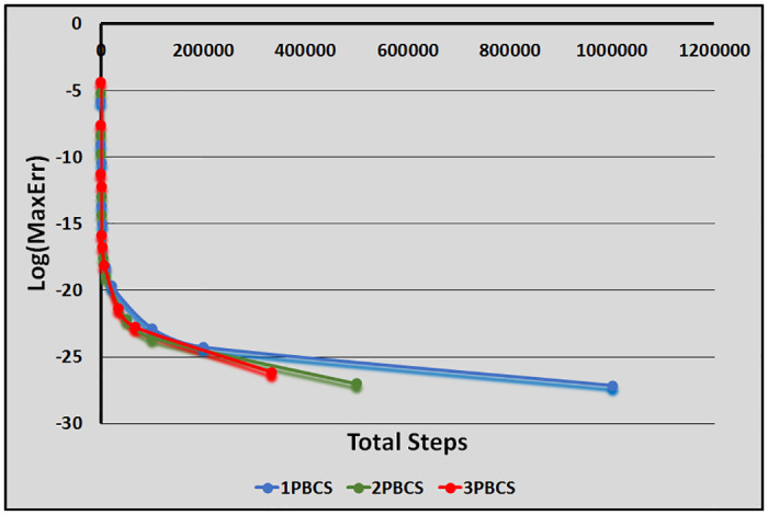
Efficiency of the 1PBCS, 2PBCS and 3PBCS methods for Example 1.
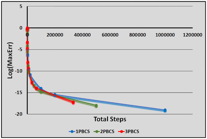
Efficiency of the 1PBCS, 2PBCS and 3PBCS methods for Example 2.
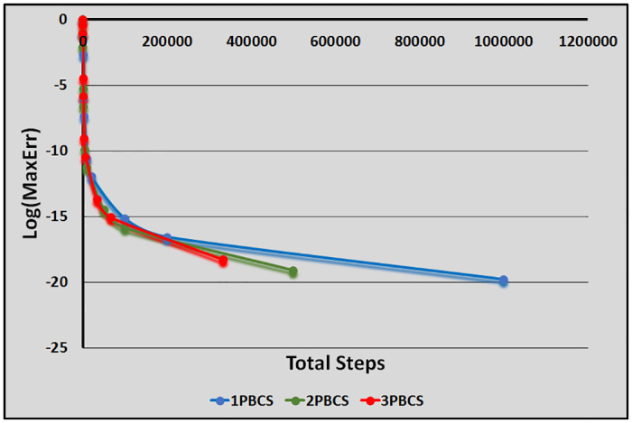
Efficiency of the 1PBCS, 2PBCS and 3PBCS methods for Example 3.

| H | Method | Example 1 | Example 2 | Example 3 | |||
|---|---|---|---|---|---|---|---|
| TSteps | ErrMax | TSteps | ErrMax | TSteps | ErrMax | ||
| 10−1 | 1PBCS | 100 | 7.45376e-01 | 100 | 1.15401e-04 | 20 | 3.21086e-01 |
| 2PBCS | 50 | 6.66935e-01 | 50 | 2.34228e-04 | 10 | 3.59297e-01 | |
| 3PBCS | 34 | 9.35380e-01 | 34 | 5.11552e-04 | 7 | 6.48511e-01 | |
| 10−2 | 1PBCS | 1000 | 8.23960e-03 | 1000 | 1.15142e-06 | 200 | 2.54695e-03 |
| 2PBCS | 500 | 1.62497e-02 | 500 | 2.30738e-06 | 100 | 5.16502e-03 | |
| 3PBCS | 334 | 3.79323e-02 | 334 | 5.17431e-06 | 67 | 1.15395e-02 | |
| 10−3 | 1PBCS | 10000 | 8.16835e-05 | 10000 | 1.15118e-08 | 2000 | 2.54180e-05 |
| 2PBCS | 5000 | 1.63524e-04 | 5000 | 2.30283e-08 | 1000 | 5.09487e-05 | |
| 3PBCS | 3334 | 3.67387e-04 | 3334 | 5.17962e-08 | 667 | 1.14395e-04 | |
| 10−4 | 1PBCSI | 100000 | 8.16543e-07 | 100000 | 1.14942e-10 | 20000 | 2.54175e-07 |
| 2PBCS | 50000 | 1.63373e-06 | 50000 | 2.30188e-10 | 10000 | 5.08467e-07 | |
| 3PBCS | 33334 | 3.67505e-06 | 33334 | 5.18013e-10 | 6667 | 1.14379e-06 | |
| 10−5 | 1PBCS | 1000000 | 5.45040e-09 | 1000000 | 1.58909e-12 | 200000 | 2.54041e-09 |
| 2PBCS | 500000 | 1.62002e-08 | 500000 | 1.86703e-12 | 100000 | 5.08386e-09 | |
| 3PBCS | 333334 | 3.58752e-08 | 333334 | 4.42069e-12 | 66667 | 1.14377e-08 | |
| H | Method | Example 1 | Example 2 | Example 3 |
|---|---|---|---|---|
| Time | Time | Time | ||
| 10−1 | 1PBCS | 3.032 | 3.032 | 3.027 |
| 2PBCS | 3.032 | 3.032 | 3.027 | |
| 3PBCS | 3.033 | 3.033 | 3.029 | |
| 10−2 | 1PBCS | 3.044 | 3.041 | 3.036 |
| 2PBCS | 3.041 | 3.037 | 3.036 | |
| 3PBCS | 3.037 | 3.035 | 3.036 | |
| 10−3 | 1PBCS | 3.049 | 3.048 | 3.052 |
| 2PBCS | 3.046 | 3.046 | 3.052 | |
| 3PBCS | 3.042 | 3.041 | 3.049 | |
| 10−4 | 1PBCSI | 3.182 | 3.192 | 3.072 |
| 2PBCS | 3.174 | 3.186 | 3.070 | |
| 3PBCS | 3.165 | 3.175 | 3.068 | |
| 10−5 | 1PBCS | 4.311 | 4.322 | 3.289 |
| 2PBCS | 4.301 | 4.310 | 3.285 | |
| 3PBCS | 4.289 | 4.298 | 3.278 |
Example 4: A 3rd order systems of ODE,

Table 3 compares results between the DI and 3PBCS methods. Opposed to the 3PBCS backward difference formulation, the DI method is derived with a divided difference formulation. The DI method was chosen to test the 3PBCS with a competing predictor-corrector multistep method. Results presented highlights maximum error (ErrEQ1, ErrEQ2, ErrEQ3) for each of equation, f1, f2 and f3 and the overall maximum error for each step size, ErrMax. The error is obtained by comparing approximated solution with the exact solution, with conditions established in (31). The DI was selected because of its divided difference formulation. The purpose was to test the performance of the 3PBCS method against an alternative multistep method using similar parameter. In the current case, both methods were set using similar order methods (same number of back values). Results of the current example clearly illustrates the advantage of 3PBCS over the DI method.
| H | Method | TSteps | ErrEQ1 | ErrEQ2 | ErrEQ3 | ErrMax |
|---|---|---|---|---|---|---|
| 10−1 | DI | 30 | 1.00000e+00 | 1.00000e+00 | 1.00000e+00 | 1.00000e+00 |
| 3PBCS | 10 | 1.00000e+00 | 1.00000e+00 | 1.00000e+00 | 1.00000e+00 | |
| 10−2 | DI | 300 | 1.00000e+00 | 1.00000e+00 | 1.00000e+00 | 1.00000e+00 |
| 3PBCS | 100 | 6.69108e-02 | 1.77349e-02 | 1.05606e-02 | 6.69108e−02 | |
| 10−3 | DI | 3000 | 8.40056e−01 | 3.82868e−01 | 1.15686e−01 | 8.40056e−01 |
| 3PBCS | 1000 | 1.98994e-04 | 1.78543e-04 | 1.22428e-04 | 1.98994e-04 | |
| 10−4 | DI | 30000 | 4.04766e−02 | 1.56457e−02 | 2.34364e−03 | 4.04766e−02 |
| 3PBCS | 10000 | 1.97238e-06 | 1.78345e-06 | 1.22641e-06 | 1.97238e-06 | |
| 10−5 | DI | 300000 | 2.31051e−03 | 1.55405e−03 | 2.24310e−04 | 2.31051e−03 |
| 3PBCS | 100000 | 1.97209e-08 | 1.78295e-08 | 1.22651e-08 | 1.97209e-08 |
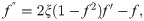
Example 5: The problem presented is a artificial second order ODE with periodic solution. The second order ODE
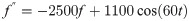
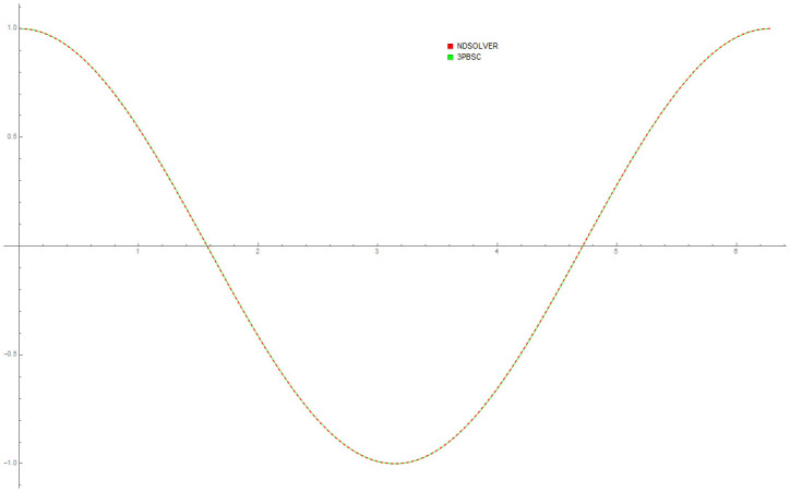
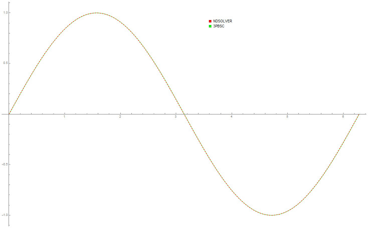
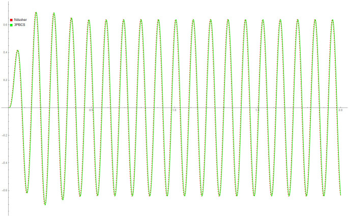
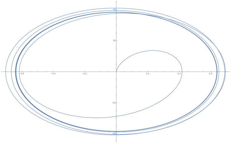
Table 4 provides numerical approximation by the 3PBCS and the provided exact solution for Example 5. Due to the difficulty of the current example, the step size of order H = 10−5 is selected. Results show a consistent approximation error of 1×10⁻⁶ for every point. To further validate the accuracy of 3PBCS as suitable method for the approximation of a non linear ODE with periodic solution, 3PBCS is compared against NDSOLVER, a preset Euler method equipped in Mathematica 12. The plotted graph displayed in Fig 4 shows that the 3PBCS method matches the solution obtained by NDSOLVER thus, confirming the accuracy of the method. Figs 5 and 6 are 2D and 3D parametric plots of Example 5 by the 3PBCS. For a clear understanding of the difficulty level for Example 5, readers may also refer to a 3D representation of the periodic solutions as illustrated in Fig 7.
Comparison between NDSOLVER and 3PBCS for the solution of Example 5.
Parametric plot of f and f′ of 3PBCS method for Example 5.
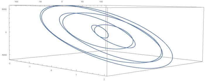
3D parametric plot of f, f′ and f″ approximated by 3PBCS method for Example 5.
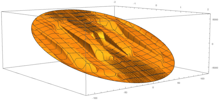
3D representation of 3PBCS method for Example 5.
| Approximate f(tn+3) | Exact fn(t) | ErrMax | |
|---|---|---|---|
| 0.5 | -2.86605e−03 | -2.86603e−03 | 1.29539e−06 |
| 1 | 6.90035e−01 | 6.90038e−01 | 2.46112e−06 |
| 1.5 | 6.02881e−02 | 6.02920e−02 | 3.85117e−06 |
| 2 | -1.32055e+00 | -1.32055e+00 | 4.36827e−06 |
Test problems in the current section are practical ODEs that are found in real applications including two body motion, thin flow and electrical circuits. Lets begin with the renowned two body motion.
Example 6: Newton’s equation of the two body motion problem refers to the movement of two particle interacting which each other due to gravitational pull, neglecting any third body the two do not collide with (see Fig 8)
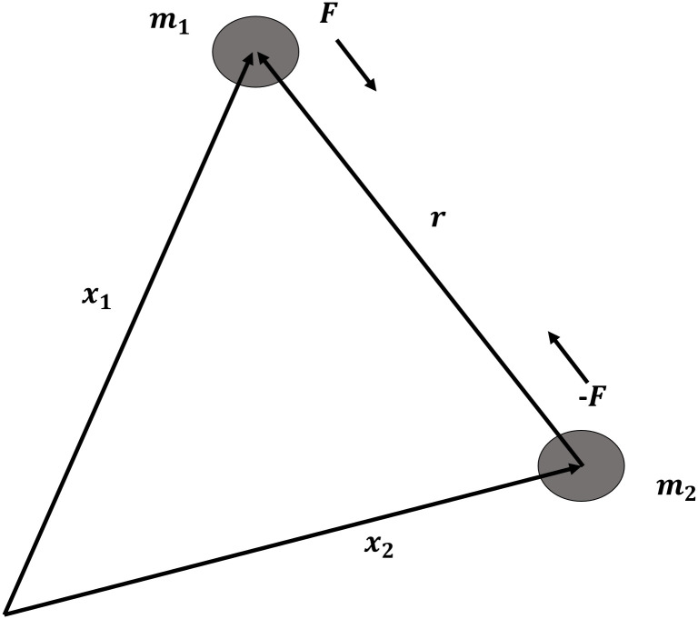
The two body problem.
In the current research, we consider the following formulation of the two body problem
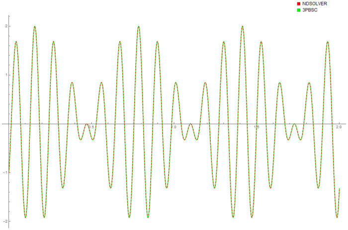
Data provided in Table 5 are numerical approximations for Example 6 using DI and 3PBCS method. Results exhibits that when using a larger step size, both methods are comparable but as smaller step size are used, 3PBCS begins showing an obvious advantage. Results produced in the table shows that the accuracy of 3PBCS improves at a rate of H2 compared to e the DI method which barely equals the current step size. To further validate the capability of the 3PBCS method, Figs 9 dan 10 show graphical approximation of f1 and f2 by NDSOLVER and 3PBCS methods. It is clear that both methods practically overlap each other, point by point. Fig 11 is presented to illustrate the orbit of the two body motion as approximated by 3PBCS. Example 6, with the current initial conditions presents a circular orbit (orbit 1), where as, by changing the initial conditions to , gives Example 6 a Kepler-like solution which produces an elliptic orbit (orbit 2) and can be verified from the work of Shampine and Gordon [37].
Comparison between NDSOLVER and 3PBCS for f1 of Example 6.
Comparison between NDSOLVER and 3PBCS for f2 of Example 6.
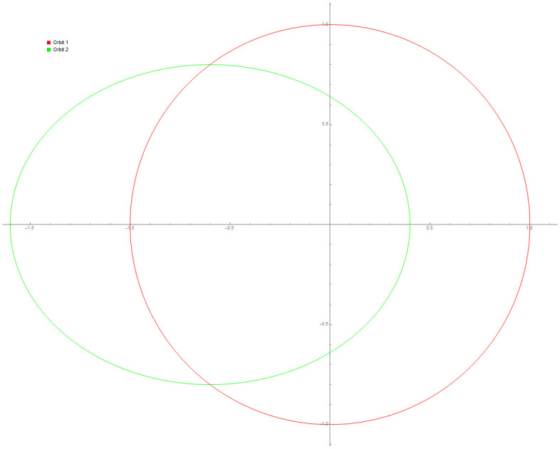
Orbit for Example 6 with different initial conditions.
| H | Example 6 | |||
|---|---|---|---|---|
| Method | TSteps | ErrEQ1 | ErrEQ2 | |
| 10−1 | DI | 100 | 7.86394e−02 | 9.00026e−02 |
| 3PBCS | 34 | 2.37337e−02 | 2.11901e−02 | |
| 10−2 | DI | 1000 | 8.02804e−03 | 9.24779e−03 |
| 3PBCS | 334 | 3.11795e−04 | 3.22462e−04 | |
| 10−3 | DI | 10000 | 8.02694e−04 | 9.28815e−04 |
| 3PBCS | 3334 | 3.20106e−06 | 3.33937e−06 | |
| 10−4 | DI | 100000 | 8.02843e−05 | 9.29075e−05 |
| 3PBCS | 33334 | 3.20816e−08 | 3.34984e−08 | |
| 10−5 | DI | 1000000 | 8.02848e−06 | 9.29096e−06 |
| 3PBCS | 333334 | 3.00597e−10 | 3.43977e−10 | |
Example 7: Many problems in engineering and physics are based on the famous thin flow of liquid which is a third order ODEs with the ideal draining flow as shown in Fig 12.
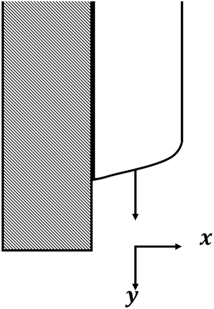
An idealized draining flow.
These thin film flow problems can be found in various form like the the infamous drainage dry surface given by the function
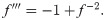


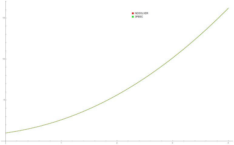
Because the thin flow problem have no exact or analytical solution, the solution by 3PBCS is compared against the solution obtained by the DI. Table 6 presents the approximated solution obtained by 3PBCS method of f, f′ and f″ for the points 1.0, 1.5, 2.0, 2.5, 3.0, 3.5 and 4.0. As shown in Table 6, both methods are comparable with similar approximation up to at least 5 decimal points. Fig 13 compares solutions by NDSOLVER and 3PBCS. For the current example, 3PBCS method approximates the solution using a step size of H = 1 × 10³. Even at the current stepsize, the figure shows 3PBCS ability to match step by step solution of the NDSOLVER. Whereas, Fig 14 illustrates the difference of solution between f, f′ and f″.
Comparison between NDSOLVER and 3PBCS for the solution of Example 6.
Numerical approximation of f, f′ and f″ by the 3PBCS method for Example 6.
| TOL | Method | k = 2 | ||
|---|---|---|---|---|
| f | f′ | f″ | ||
| 1.0 | DI | 2.60828e+00 | 2.28486e+00 | 1.46992e-01 |
| 3PBCS | 2.60828e+00 | 2.28491e+00 | 1.46992e-01 | |
| 1.5 | DI | 3.93278e+00 | 3.01725e+00 | 6.46548e-02 |
| 3PBCS | 3.93278e+00 | 3.01725e+00 | 6.46548e-02 | |
| 2.0 | DI | 5.62831e+00 | 3.76676e+00 | 3.15678e-02 |
| 3PBCS | 5.62831e+00 | 3.76677e+00 | 3.15678e-02 | |
| 2.5 | DI | 7.70090e+00 | 4.52454e+00 | 1.68623e-02 |
| 3PBCS | 7.70090e+00 | 4.52454e+00 | 1.68623e-02 | |
| 3.0 | DI | 1.01536e+01 | 5.28668e+00 | 9.69980e-03 |
| 3PBCS | 1.01536e+01 | 5.28669e+00 | 9.69979e-03 | |
| 3.5 | DI | 1.29880e+01 | 6.05132e+00 | 5.92811e-03 |
| 3PBCS | 1.29880e+01 | 6.05132e+00 | 5.92811e-03 | |
| 4.0 | DI | 1.62051e+01 | 6.81747e+00 | 3.80798e-03 |
| 3PBCS | 1.62051e+01 | 6.81747e+00 | 3.80798e-03 | |
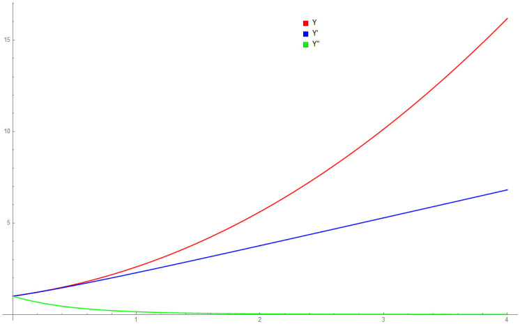
Example 8: Consider the second order RLC circuit in Fig 15 below, with resistance of 2 ohm, capacitor at and inductor at 0.1 Henry and electrical force of 100 sin 60tV. The objective is to find the capacitor charge at any time, t > 0 given the initial current and initial charge of the capacitor are both zero. By Kirchhoff law, the following second order differential equation can be derived,

Second order RLC circuit.
The following Table 7 contains numerical results of 3PBCS method for example. The approximated values for end points (Tn) 0.5, 1.0, 1.3 and 2.0 are provided with the corresponding exact solutions. The maximum error of all points, ErrMax is defined by T0 ≤ |f(tn+b) − f(t)| ≤ Tn, b = 1, 2, 3 is also provided for a clearer view of 3PBCS abilities. As demonstrated in Table 6, 3PBCS is consistently accurate to the seventh decimal point when applying a stepsize of H = 1 × 10⁻³. Fig 16 is the approximate solution for fn by NDSOLVER and 3PBCS. The graphical overlap shown in the figure exhibits the similar accuracy of both methods, whereas Fig 17 is parametric plot of Example 8 presented to express the level of difficulty of the problem.
Comparison between NDSOLVER and 3PBCS for the solution of Example 7.
Parametric plot of f and f′ of 3PBCS method for Example 7.
| Approximate f(tn+3) | Exact fn(t) | ErrMax T0 ≤ |f(tn+b) − fn(t)| ≤ Tn | |
|---|---|---|---|
| 0.5 | 3.31828e-01 | 3.31828e-01 | 1.82051e-07 |
| 1 | 5.93337e-01 | 5.93337e-01 | 1.82051e-07 |
| 1.5 | -1.46028e-01 | -1.46028e-01 | 1.82051e-07 |
| 2 | -6.38372e-01 | -6.38372e-01 | 1.82051e-07 |
Example 9: The Van der Pol equation is an ODE that is derived from Rayleigh differential equation. In a Van der Pol equation,
Example 9 is originally a problem obtained from [42]. The Van Der Pol equation selected does not have any known analytical solution. Table 8 provides approximated values of f, f′ and f″ for 5 different end points by the DI and 3PBCS methods. Numerical approximation shows that both methods obtained similar values for f, f′ and f″ up to 1 × 10⁻⁵. Figs 18 and 19 illustrate the approximated solution, f by the 3PBCS method against NDSOLVER for the interval 0 ≤ t ≤ 40. Results in Fig 18 shows similar approximation for both 3PBCS and NDSOLVER where Fig 19 illustrates a graphical representation approximated values of t against f, f′ and f″. Fig 20 is to present a 3D illustration of f, f′ and f″ which corresponds to similar steps points by the 3PBCS method.
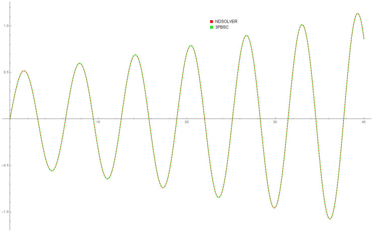
Numerical Comparison between NDSOLVER and 3PBCS.
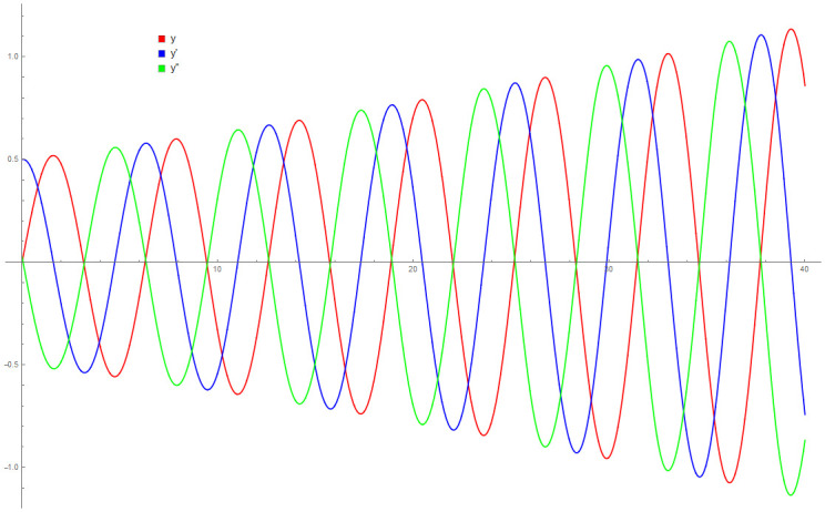
Aprroximation of f, f′ and f″ by 3PBCS method.
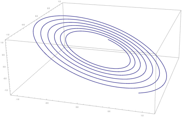
A 3D parametric plot of f, f′ and f″ approximated by 3PBCS method for Example 5.
| Tn | Method | f | f′ | f″ |
|---|---|---|---|---|
| 0.5 | DI | 2.4270367281e-001 | 4.5018020968e-001 | -2.2152055722e-001 |
| 3PBCS | 2.4270367388e-001 | 4.5018022195e-001 | -2.2152055773e-001 | |
| 1.0 | DI | 4.3105071043e-001 | 2.8664149615e-001 | -4.1938160270e-001 |
| 3PBCS | 4.3105073032e-001 | 2.8664156431e-001 | -4.1938162006e-001 | |
| 1.5 | DI | 5.1671714810e-001 | 4.8026186062e-002 | -5.1495698025e-001 |
| 3PBCS | 5.1671722009e-001 | 4.8026324566e-002 | -5.1495704734e-001 | |
| 2.0 | DI | 4.7630950304e-001 | -2.0708952836e-001 | -4.8431485170e-001 |
| 3PBCS | 4.7630965708e-001 | -2.0708934721e-001 | -4.8431499722e-001 | |
| 2.5 | DI | 3.1729761641e-001 | -4.1655545180e-001 | -3.3602849515e-001 |
| 3PBCS | 3.1729786006e-001 | -4.1655528657e-001 | -3.3602872814e-001 | |
| 5.0 | DI | -5.3857425618e-001 | 1.4704130967e-001 | 5.4379376516e-001 |
| 3PBCS | -5.3857445794e-001 | 1.4704079637e-001 | 5.4379394710e-001 |
Results provided in the current work validate that 3PBCS is a viable numerical method for solving ODEs. The three-point element of the method allows for lesser computational cost and provides better efficiency compared to its rival counterparts. By simply using a constant step size algorithm decreases computational cost and increases efficiency. Tables 1, 3 and 5 validate the convergence of the method. When a smaller H is selected, the method becomes more accurate and proven to provide a consistent set of accuracy for every point in the interval as indicated in Tables 4 and 7. For future works, the 3PBCS can be fitted with a variable order step size and parallel computing algorithm. The effectiveness of a variable order step size algorithm depends on the selection of a suitable order step size criterion. Authors a currently refining appropriate conditions to provide a better approximation for a variable order step size algorithm.
We would like to thank both Universiti Sains Islam Malaysia and Universiti Putra Malaysia for fully supporting our efforts and assisting us in completing this research.
1
2
3
4
5
6
7
8
9
10
11
12
13
14
15
16
17
18
19
20
21
22
23
24
25
26
27
28
29
30
31
32
33
34
35
36
37
38
39
40
41
42
 Approximating non linear higher order ODEs by a three point block algorithm
 Facebook
 Twitter
 Linkedin
 Whatsapp

