A new CUSUM control chart under uncertainty with applications in petroleum and meteorology

Muhammad Aslam, Ambreen Shafqat, Mohammed Albassam, Jean-Claude Malela-Majika, Sandile C. Shongwe

Competing Interests: The authors have declared that no competing interests exist.

https://doi.org/10.1371/journal.pone.0246185, Volume: 16, Issue: 2, Pages: 1-16

Article Type: research-article Article History

Publisher: Public Library of Science

- Facebook
- Twitter
- Linkedin
- Whatsapp
Altmetric

Table of Contents

Introduction
Conclusion and future recommendations

Abstract

In these last few decades, control charts have received a growing interest because of the important role they play by improving the quality of the products and services in industrial and non-industrial environments. Most of the existing control charts are based on the assumption of certainty and accuracy. However, in real-life applications, such as weather forecasting and stock prices, operators are not always certain about the accuracy of an observed data. To efficiently monitor such processes, this paper proposes a new cumulative sum (CUSUM) X¯

chart under the assumption of uncertainty using the neutrosophic statistic (NS). The performance of the new chart is investigated in terms of the neutrosophic run length properties using the Monte Carlo simulations approach. The efficiency of the proposed neutrosophic CUSUM (NCUSUM) X¯

chart is also compared to the one of the classical CUSUM X¯

chart. It is observed that the NCUSUM X¯

chart has very interesting properties compared to the classical CUSUM X¯

chart. The application and implementation of the NCUSUM X¯

chart are provided using simulated, petroleum and meteorological data.

Aslam,Shafqat,Albassam,Malela-Majika,Shongwe,and Pamucar: A new CUSUM control chart under uncertainty with applications in petroleum and meteorology

Introduction

Control charts play an essential role in monitoring processes in the production and manufacturing sectors. Shewhart-type control charts are the most popular charts because of its simplicity and attractive sensitivity towards large shifts in the process parameters. These charts are widely applied in many fields and operations (such as manufacturing processes, health care monitoring, stock exchange, credit card, financial fraud detection, weather updates, and internet traffic flow, etc.). However, Shewhart-type charts are inefficient in detecting small to moderate process shifts. Due to this drawback, researchers have developed new control charts based on classical and adaptive sampling designs to detect small-to-moderate process shifts as quickly as possible, including large shifts. Control charts are classified into memory-type (e.g. cumulative sum (CUSUM), exponentially weighted moving average (EWMA), etc.) and memoryless (e.g. Shewhart-type) control charts; see for instance [1]. The latter uses only the latest information of the process to compute the charting statistics, which makes it less sensitive to detect small-to-moderate shifts, but enhances its ability to detect large shifts in the process. The first (i.e. memory-type control chart) uses both current and past information to compute the charting statistics, which makes it more sensitive in detecting small-to-moderate shifts and less sensitive in detecting large shifts in the process. The CUSUM and EWMA charts are the most popular memory-type control charts. To enhance the aforementioned charts, various advanced techniques are used including the addition of run rules, the use of variable sampling interval (VSI) and variable sample size (VSS) sampling designs for adaptive charts. Among all the advanced developments in the statistical process control (SPC) field, the CUSUM chart is an efficient alternative to the Shewhart chart when it comes to the detection of small to moderate shifts, see [1].

Both memory-type and memory-less control charts are used to monitor and control the spread or location parameters in any process. The sensitivity of memory-type charts have attracted the attention of many researchers and brought many more improvements in the SPC field and management of many organizations. Due to the efficiency of the CUSUM and EWMA charts, many other control charts have been developed. Lucas and Crosier [2] incorporated a fast initial response (FIR) feature to the classical CUSUM and compared its performance to that of the classical CUSUM chart. Zhao et al. [3] developed a dual CUSUM scheme which combines two CUSUM chart to detect a small shift in a process. Li and Wang [4] proposed an adaptive CUSUM Q chart also known as the self-starting approach. Shafqat et al. [5] introduced a linear prediction model based on the double EWMA control chart for non-normal situations for monitoring the location parameter. Haq [6] and Haq et al. [7, 8] proposed the use of EWMA control charts to monitor various processes, i.e. the mean and variance using ranked set sampling and the mean under the effect of measurement errors using ranked set sampling. Sanusi et al. [9] introduced a different approach for the EWMA-based chart when supplementary information about the main variable is not constant. Some different applications of attributes and variables control charts can be found in [10, 11].

The classical Shewhart control charts cannot be used efficiently when data are collected from uncertain and random situations, or when there are inconsistencies in the collected data. Khademi and Amirzadeh [12] reported that “fuzzy data exist ubiquitously in the modern manufacturing processes”; hence, in certain monitoring environments, ‘fuzzy model’ control charts are preferred when parameters or observations are uncertain, see for instance [13]. Senturk and Erginel [14] introduced the dispersion control chart by using the fuzzy logic, and Faraz et al. [15] proposed a control chart combining uncertainty and randomness assumptions. Smarandache [16] provided an overview of the fuzzy logic and reported that the neutrosophic logic deals efficiently with indeterminacy. In [17, 18], the neutrosophic logic is used to develop the idea of the neutrosophic statistics. Neutrosophic statistics is an extension of the classical statistics that is more efficient in analyzing data from ambiguous environment. For publications on neutrosophic statistics applied in various fields of knowledge, the readers are referred to [19–21]. For non-normal processes, control charts with a fuzzy approach are discussed by [22]. Pereira et al. [23] designed a fuzzy chart for monitoring the blood components under the violation of the normality assumption. The most recent research works on control charts that use neutrosophic statistics concepts, can be found in [24–28].

At the best of the authors’ knowledge, there is no work on the CUSUM control chart under neutrosophic statistics. In this paper, the CUSUM $\bar{X}$ control chart using the neutrosophic statistical method is proposed. Following the reports in [16, 17], it is presumed that the proposed neutrosophic CUSUM (NCUSUM) $\bar{X}$ chart will provide very interesting properties (i.e. will be more efficient in detecting a small shift in the process and more informative, flexible, and effective in uncertain conditions).

The rest of this paper is structured as follows: The second section gives a brief description of the classical CUSUM $\bar{X}$ chart and an introduction to the NCUSUM $\bar{X}$ control chart. In the third section, the performance of the proposed NCUSUM $\bar{X}$ chart is extensively investigated in terms of the neutrosophic run length properties. Moreover, the performance of the proposed chart is compared with the classical CUSUM $\bar{X}$ chart. Fourth and fifth sections provide illustrative applications of the new chart using simulated and real-life datasets, respectively. The conclusion and recommendations are given in the last section.

The CUSUM control chart

The classical CUSUM chart

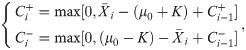
The CUSUM $\bar{X}$ chart for monitoring small and moderate shifts in the mean was first introduced by [29]. The two-sided CUSUM chart is used to monitor upwards and downward shifts in the process parameters using the charting statistics $C_{i}^{+}$ and $C_{i}^{-}$ , respectively, where i represents the sample number (or sampling time). Assume that X is a sequence of independent normally distributed observations given that the in-control mean μ₀ and variance $σ_{0}^{2}$ ; thus, the charting statistics of the two-sided CUSUM $\bar{X}$ chart (i.e. $C_{i}^{+}$ and $C_{i}^{-}$ , with $C_{0}^{+} = C_{0}^{-} = 0$ ) are plotted versus a single control limit denoted by H. These charting statistics are mathematically defined by

where

\bar{X}

is the sample mean, μ₀ is the target mean value of X and K is the reference value. The CUSUM chart depends on two singleton parameters, i.e. K and H, which need to be selected carefully because the sensitivity of the CUSUM chart depend on them, see pages 404–405 of Montgomery []. These parameters are chosen such that:

where

V a r (\bar{X}) = σ_{X}^{2} / n, σ_{X}^{2}

is the variance of X, k is selected to be half of the shift (i.e.

k = \frac{δ}{2}

, with δ is the shift in standard deviation units) and h is usually selected to be approximately five times the standard deviation units. Note that the process has moved upwards if

C_{i}^{+} > H

for any value of i; however, if

C_{i}^{-} > H

, the process has moved downwards.

In the next sub-section, the proposed NCUSUM $\bar{X}$ chart is introduced using the framework of the classical CUSUM $\bar{X}$ chart.

The proposed neutrosophic CUSUM chart

In the uncertain environments having inconsistency data, the quality characteristic of interest (denoted by X_Ni) is not a deterministic value; hence, it falls within some interval, say [X_Li, X_Ui], where the subscripts L and U refers to the lower and upper bound of those particular values; for instance, X_Li is a lower bound of X_Ni and X_Ui is the upper bound of X_Ni (i.e. X_Li≤X_Ni≤X_Ui). The latter lower and upper notation holds for other expressions defined in this subsection. That is, the neutrosophic quality characteristic of interest X_Ni; X_Ni∈[X_Li, X_Ui], follows neutrosophic normal distribution with neutrosophic mean μ_0N; μ_0N∈[μ_L, μ_U] and neutrosophic variance $σ_{0 N}^{2}; σ_{0 N}^{2} \in [σ_{L}^{2}, σ_{U}^{2}]$ , with μ_L≤μ_U and $σ_{L}^{2} \leq σ_{U}^{2}$ . Hence, the sample mean of the variable X_Ni is given by ${\bar{X}}_{N i} \in [{\bar{X}}_{L i}, {\bar{X}}_{U i}]$ , $V a r ({\bar{X}}_{N i}) = \frac{σ_{N i}^{2}}{n_{N}}; n_{N} \in [n_{L}, n_{U}]$ with n_L≤n_U, σ_Ni∈[σ_Li, σ_Ui] is the observed neutrosophic standard deviation of X_iN, with σ_Li≤σ_Ui. Thus, the plotting statistics of the proposed NCUSUM $\bar{X}$ chart under uncertain environments is given by

where

M_{N i}^{+} \in [M_{L i}^{+}, M_{U i}^{+}]

M_{N i}^{-} \in [M_{L i}^{-}, M_{U i}^{-}]

, K_N∈[K_L, K_U], H_N∈[H_L, H_U] and μ_0N is the target mean value. In addition, μ_1N = μ_0N+δσ_0N, where μ_0N∈[μ_0L, μ_0U] and μ_1N∈[μ_1L, μ_1U] represents the in-control and out-of-control neutrosophic mean, respectively; with δ denoting the shift in the mean. Moreover,

where k_N and h_N are the design parameters of the proposed NCUSUM

\bar{X}

chart. The initial values for the plotting statistics which are given in Eq () are equal to zero, i.e.

M_{N 0}^{+} = M_{N 0}^{-} = 0

. The plotting statistics of the proposed chart are plotted versus the control limit H_N. The evaluation rule for the proposed chart is given as: for any value of i, if the value of

M_{N i}^{+} > H_{N}

then the process of the mean is declared to have shifted upward; otherwise, if the value of

M_{N i}^{-} > H_{N}

then the process mean is declared to have moved downward. The values of k_N and h_N need to be selected with caution because the run length (RL) properties of the chart depend on them. Note that the RL is the number of charting statistics that are required before the first out-of-control signal is issued by a control chart. The manner in which the design parameters k_N and h_N are obtained is discussed in the next section.

Run length performance

Performance of the NCUSUM $\bar{X}$ chart

For some selected values of k_N and n_N, for example k_N∈{[0.20,0.25], [0.4,0.5]}, and n_N∈{[3,5],[10,20]}, the corresponding values of h_N are found by running 10⁵ simulations in R software for some given fixed nominal neutrosophic average RL (denoted by NARL₀) values of 300, 370, 400, 500. Tables 1–3 display the in-control and out-of-control neutrosophic average and standard deviation of the RL (denoted as NARL and NSDRL) profiles of the proposed chart using different parameters, where NARL∈[NARL_L, NARL_U] and NSDRL∈[NSDRL_L, NSDRL_U], with NARL_L≤NARL_U and NSDRL_L≤NSDRL_U. In other words, Tables 1–3 give the ideal combinations of h_N and k_N when the nominal NARL₀ values are 300, 370, 400 and 500 for different values of n_N.

Table 1

The NARL and NSDRL values of the proposed NCUSUM

\bar{X}

chart when n_N∈[3, 5], k_N∈[0.20, 0.25] for different nominal NARL.

NARL	300		370		400		500
h_N	[7.602,8.662]		[8.099,9.299]		[8.319,9.499]		[9.039,10.299]
δ	NARLs	NSDRLs	NARLs	NSDRLs	NARLs	NSDRLs	NARLs	NSDRLs
0	[301.07,301.18]	[271.92,283.10]	[370.28,371.70]	[330.58,342.12]	[400.39,401.79]	[360.15,371.83]	[500.44,501.54]	[441.99,447.12]
0.25	[22.74,32.70]	[12.50,19.00]	[24.94,35.23]	[13.38,20.73]	[25.64,36.61]	[13.68,20.68]	[27.04,40.06]	[14.01,22.71]
0.5	[9.11,13.77]	[3.38,5.35]	[9.77,14.57]	[3.32,5.38]	[10.20,15.04]	[3.49,5.47]	[11.15,15.74]	[3.61,5.58]
0.75	[5.00,8.59]	[1.61,2.56]	[6.36,9.33]	[1.75,2.80]	[6.54,9.52]	[1.77,2.66]	[6.96,10.14]	[1.76,2.78]
1	[4.24,6.27]	[1.06,1.60]	[4.68,6.67]	[1.09,1.69]	[4.82,6.87]	[1.06,1.71]	[5.20,7.36]	[1.15,1.71]
1.5	[2.99,4.21]	[0.58,0.87]	[3.17,4.51]	[0.57,0.87]	[3.24,4.51]	[0.61,0.89]	[3.44,4.86]	[0.61,0.91]
2	[2.25,3.22]	[0.44,0.57]	[2.44,3.38]	[0.50,0.60]	[2.46,3.42]	[0.51,0.59]	[2.67,3.70]	[0.51,0.60]
2.5	[1.99,2.60]	[0.33,0.51]	[2.03,2.81]	[0.29,0.56]	[2.03,2.84]	[0.20,0.56]	[2.14,3.03]	[0.34,0.49]
3	[1.87,2.18]	[0.15,0.38]	[1.96,2.29]	[0.19,0.45]	[1.96,2.38]	[0.17,0.46]	[1.99,2.60]	[0.29,0.39]
4	[1.15,1.97]	[0.16,0.35]	[1.26,1.99]	[0.08,0.43]	[1.36,2.00]	[0.09,0.44]	[1.62,2.01]	[0.18,0.30]
5	[1.00,1.57]	[0.00,0.29]	[1.00,1.80]	[0.03,0.39]	[1.00,1.85]	[0.05,0.40]	[1.02,1.96]	[0.15,0.25]
6	[1.00,1.07]	[0.00,0.16]	[1.00,1.20]	[0.00,0.20]	[1.00,1.22]	[0.01,0.22]	[1.00,1.55]	[0.00,0.23]
7	[1.00,1.00]	[0.00,0.03]	[1.00,1.00]	[0.00,0.07]	[1.00,1.00]	[0.00,0.09]	[1.00,1.03]	[0.00,0.12]

Table 2

The NARL and NSDRL values of the proposed NCUSUM

\bar{X}

chart when n_N∈[3, 5], k_N∈[0.4, 0.5] for different nominal NARL.

NARL₀	300		370		400		500
h_N	[4.585,5.421]		[4.787,5.751]		[4.887,5.894]		[5.179,6.314]
δ	NARLs	NSDRLs	NARLs	NSDRLs	NARLs	NSDRLs	NARLs	NSDRLs
0	[301.20,301.83]	[292.12,299.37]	[370.88,371.32]	[354.69,355.21]	[400.82,401.85]	[370.48,374.30]	[501.32,501.62]	[450.81,452.90]
0.25	[25.76,35.74]	[20.24,27.67]	[28.53,41.29]	[22.35,32.16]	[28.51,43.22]	[21.76,33.36]	[31.94,48.29]	[25.25,37.55]
0.5	[8.07,12.05]	[4.07,6.65]	[8.27,12.84]	[4.07,6.84]	[8.38,13.11]	[2.98,6.43]	[9.13,13.70]	[4.53,6.49]
0.75	[4.61,6.67]	[1.74,2.60]	[4.70,7.09]	[1.69,2.72]	[4.87,7.20]	[1.77,2.68]	[5.08,7.65]	[1.78,2.91]
1	[3.27,4.79]	[0.99,1.64]	[3.35,5.06]	[0.99,1.64]	[3.41,5.15]	[1.04,1.69]	[3.55,5.46]	[1.04,1.63]
1.5	[2.17,3.04]	[0.47,0.81]	[2.24,3.15]	[0.52,0.81]	[2.25,3.28]	[0.52,0.79]	[2.35,3.51]	[0.55,0.86]
2	[1.74,2.29]	[0.45,0.51]	[1.81,2.43]	[0.40,0.53]	[1.85,2.45]	[0.40,0.55]	[1.91,2.61]	[0.36,0.58]
2.5	[1.32,1.98]	[0.32,0.46]	[1.36,2.03]	[0.32,0.48]	[1.43,2.05]	[0.30,0.32]	[1.49,2.12]	[0.30,0.37]
3	[1.04,1.74]	[0.19,0.43]	[1.08,1.82]	[0.27,0.38]	[1.08,1.86]	[0.27,0.34]	[1.15,1.93]	[0.25,0.30]
4	[1.00,1.12]	[0.00,0.33]	[1.00,1.21]	[0.00,0.20]	[1.02,1.26]	[0.00,0.30]	[1.00,1.42]	[0.09,0.19]
5	[1.00,1.00]	[0.00,0.00]	[1.00,1.00]	[0.00,0.07]	[1.00,1.01]	[0.00,0.09]	[1.00,1.02]	[0.00,0.06]
6	[1.00,1.00]	[0.00,0.00]	[1.00,1.00]	[0.00,0.00]	[1.00,1.00]	[0.00,0.00]	[1.00,1.00]	[0.00,0.00]
7	[1.00,1.00]	[0.00,0.00]	[1.00,1.00]	[0.00,0.00]	[1.00,1.00]	[0.00,0.00]	[1.00,1.00]	[0.00,0.00]

Table 3

The NARL and NSDRL values of the proposed NCUSUM

\bar{X}

chart when n_N∈[10, 20], k_N∈[0.4, 0.5] for different nominal NARL.

NARL₀	300		370		400		500
h_N	[5.478,7.389]		[4.804,5.730]		[4.917,5.859]		[5.224,6.172]
δ	NARLs	NSDRLs	NARLs	NSDRLs	NARLs	NSDRLs	NARLs	NSDRLs
0	[301.10,301.60]	[282.31,301.61]	[370.27,370.54]	[353.60,359.17]	[401.29,401.47]	[374.27,385.41]	[500.08,501.92]	[453.29,460.42]
0.25	[12.32,13.55]	[3.84,6.87]	[8.43,14.49]	[4.28,8.06]	[8.50,14.96]	[4.02,7.65]	[9.09,15.13]	[4.12,7.73]
0.5	[4.89,5.46]	[0.97,1.80]	[3.45,5.51]	[1.06,1.94]	[3.47,5.65]	[1.01,1.88]	[3.67,6.11]	[1.08,2.07]
0.75	[3.16,3.29]	[0.49,0.94]	[2.23,3.50]	[0.51,0.90]	[2.27,3.62]	[0.49,0.96]	[2.39,3.74]	[0.56,0.99]
1	[2.32,2.86]	[0.45,0.61]	[1.81,2.67]	[0.41,0.61]	[1.84,2.68]	[0.40,0.64]	[1.92,2.79]	[0.33,0.65]
1.5	[1.63,1.87]	[0.23,0.34]	[1.08,1.95]	[0.27,0.37]	[1.09,1.94]	[0.28,0.58]	[1.17,2.00]	[0.25,0.37]
2	[1.02,1.14]	[0.00,0.27]	[1.00,1.41]	[0.03,0.25]	[1.00,1.49]	[0.00,0.50]	[1.00,1.58]	[0.00,0.49]
2.5	[1.00,1.00]	[0.00,0.14]	[1.00,1.06]	[0.00,0.20]	[1.00,1.04]	[0.00,0.20]	[1.00,1.09]	[0.00,0.28]
3	[1.00,1.00]	[0.00,0.00]	[1.00,1.00]	[0.00,0.03]	[1.00,1.00]	[0.00,0.04]	[1.00,1.00]	[0.00,0.03]
4	[1.00,1.00]	[0.00,0.00]	[1.00,1.00]	[0.00,0.00]	[1.00,1.00]	[0.00,0.00]	[1.00,1.00]	[0.00,0.00]
5	[1.00,1.00]	[0.00,0.00]	[1.00,1.00]	[0.00,0.00]	[1.00,1.00]	[0.00,0.00]	[1.00,1.00]	[0.00,0.00]
6	[1.00,1.00]	[0.00,0.00]	[1.00,1.00]	[0.00,0.00]	[1.00,1.00]	[0.00,0.00]	[1.00,1.00]	[0.00,0.00]
7	[1.00,1.00]	[0.00,0.00]	[1.00,1.00]	[0.00,0.00]	[1.00,1.00]	[0.00,0.00]	[1.00,1.00]	[0.00,0.00]

The following algorithm was applied to determine the values of k_N and n_N.

Step-1: specify the values of NARL₀ and n_N.

Step-2: Determine the values of k_N and n_N where NARL≥NARL₀. Chose the values of k_N and n_N where NARL is very close or exact to NARL₀.

Step-3: Determine the values of NARLs and NSDRLs for various values of δ.

The performance of the proposed NCUSUM $\bar{X}$ control chart is evaluated in terms of different RL criteria, i.e. NARLs, NSDRL and the percentiles of the run length (PRL), i.e. the 25^th, 50^th and 75^th percentiles which are denoted by P25 (i.e. P25∈[P25_L, P25_U]), P50 (i.e. P50∈[P50_L, P50_U]) and P75 (i.e. P75∈[P75_L, P75_U]). The following analysis would be noticed through Tables 1–6:

Tables 1–5 show that there are inverse relationships between the values of out-of-control NARL (denoted as NARL₁) and the values of δ. That is, the smallest value of NARL₁ is found at the largest values of δ, i.e. [1.00,1.00]. In other words, as δ increase, the values of NARL₁ decrease until they approach a value of one, i.e. [1.00,1.00]. The latter implies that, for large values of δ, the control chart will give an out-of-control signal on the next sampling point. Similarly, the NSDRLs tend to zero for largest values of δ, i.e. [0.00,0.00], which means that the variability is reduced when δ values are large.

For a specified neutrosophic sample size, n_N, there is an increasing trend in NARL₁ values as the neutrosophic value of k_N increase at small shifts of δ; however, there is an decreasing trend in NARL₁ values for large shifts of δ (see Tables 1 and 2). For instance, when k_N∈[0.20,0.25], n_N∈[3,5] and δ = 0.25 for a NARL₀ = 370, the NARL₁∈[24.94,35.23]; however, when k_N∈[0.40,0.50], the NARL₁∈[28.53,41.29] using the same parameters. Note though, at δ = 3 for the same NARL₀ value, the NARL₁ is equal to [1.96,2.29] and [1.08,1.82] for k_N equal to [0.20,0.25] and [0.40,0.50], respectively. Moreover, when design parameters are kept fixed, as δ increase, there is a decrease in the values of NARL₁.

From Tables 2 and 3, it can be noticed that the NARL₁ decreases rapidly when n_N increase, with the restriction for the value of [k_L, k_U] being constant. For instance, when δ = 0.25 and [k_L, k_U] = [0.40,0.50] for a nominal NARL₀ = 370, the NARL₁ is equal to [28.53,41.29] and [8.43,14.49] when n_N is equal to [3,5] and [10,20], respectively. This indicates improving detection ability.

The in-control neutrosophic RL distribution of the proposed chart is positively skewed as the in-control NARL are greater than the in-control P50. For instance, for the design parameters k_N∈[0.20,0.25] and n_N∈[3,5] corresponding to δ = 0, the in-control values of the P50∈[273,277] are smaller than NARL₀ = 370 (see for instance Tables 1–6). The latter implies that the distribution of the NCUSUM $\bar{X}$ chart is positively skewed.

Regardless of the NARL₀ value, the sensitivity of the NCUSUM $\bar{X}$ chart increase rapidly as δ increases in terms of the P25, P50 and P75 values, see Tables 4–6.

Table 4

The neutrosophic percentile points of the proposed NCUSUM

\bar{X}

chart when n_N∈[3, 5], k_N∈[0.20, 0.25] for different nominal NARL.

NARL₀	300		370		400		500
δ	P25	P50	P25	P75	P50	P75	P25	P50
0	[98,104]	[220,230]	[111,123]	[399,420]	[273,277]	[502,518]	[119,132]	[293,294]
0.25	[14,19]	[21,28]	[15,21]	[28,41]	[22,30]	[31,44]	[16,22]	[23,31]
0.5	[7,10]	[9,13]	[7,11]	[11,17]	[9,14]	[12,18]	[8,11]	[10,14]
0.75	[5,7]	[6,8]	[5,7]	[7,10]	[6,9]	[7,11]	[5,8]	[6,9]
1	[4,5]	[4,6]	[4,5]	[5,7]	[5,6]	[5,8]	[4,6]	[5,7]
1.5	[3,4]	[3,4]	[3,4]	[3,5]	[3,4]	[3,5]	[3,4]	[3,4]
2	[2,3]	[2,3]	[2,3]	[3,4]	[2,3]	[3,4]	[2,3]	[2,3]
2.5	[2,2]	[2,3]	[2,3]	[2,3]	[2,3]	[2,3]	[2,3]	[2,3]
3	[2,2]	[2,2]	[2,2]	[2,2]	[2,2]	[2,3]	[2,2]	[2,2]
4	[1,2]	[1,2]	[1,2]	[1,2]	[1,2]	[2,2]	[1,2]	[1,2]
5	[1,1]	[1,2]	[1,2]	[1,2]	[1,2]	[1,2]	[1,2]	[1,2]
6	[1,1]	[1,1]	[1,1]	[1,1]	[1,1]	[1,1]	[1,1]	[1,1]
7	[1,1]	[1,1]	[1,1]	[1,1]	[1,1]	[1,1]	[1,1]	[1,1]

Table 5

The neutrosophic percentile points of the proposed NCUSUM

\bar{X}

chart when n_N∈[3, 5], k_N∈[0.4, 0.5] for different nominal NARL.

NARL₀	300		370		400		500
δ	P25	P50	P25	P75	P50	P75	P25	P50
0	[87,91]	[201,202]	[109,109]	[405,428]	[264,268]	[504,528]	[120,120]	[285,293]
0.25	[12,17]	[19,27]	[12,18]	[34,47]	[22,33]	[37,54]	[13,19]	[22,33]
0.5	[5,7]	[7,10]	[5,8]	[10,15]	[7,11]	[10,16]	[6,8]	[7,12]
0.75	[3,5]	[4,6]	[3,5]	[6,8]	[4,7]	[6,8]	[4,5]	[5,7]
1	[3,4]	[3,5]	[3,4]	[4,6]	[3,5]	[4,6]	[3,4]	[3,5]
1.5	[2,3]	[2,3]	[2,3]	[2,3]	[2,3]	[3,4]	[2,3]	[2,3]
2	[1,2]	[2,2]	[2,2]	[2,3]	[2,2]	[2,3]	[2,2]	[2,2]
2.5	[1,2]	[1,2]	[1,2]	[2,2]	[1,2]	[2,2]	[1,2]	[1,2]
3	[1,1]	[1,2]	[1,2]	[1,2]	[1,2]	[1,2]	[1,2]	[1,2]
4	[1,1]	[1,1]	[1,1]	[1,1]	[1,1]	[1,1]	[1,1]	[1,1]
5	[1,1]	[1,1]	[1,1]	[1,1]	[1,1]	[1,1]	[1,1]	[1,1]
6	[1,1]	[1,1]	[1,1]	[1,1]	[1,1]	[1,1]	[1,1]	[1,1]
7	[1,1]	[1,1]	[1,1]	[1,1]	[1,1]	[1,1]	[1,1]	[1,1]

Table 6

The neutrosophic percentile points of the proposed NCUSUM

\bar{X}

chart when n_N∈[10, 20], k_N∈[0.4, 0.5] for different nominal NARL.

NARL₀	300		370		400		500
δ	P25	P50	P25	P75	P50	P75	P25	P50
0.00	[89,90]	[201,205]	[111,114]	[408,408]	[250,251]	[511,547]	[120,121]	[275,276]
0.25	[5,8]	[7,12]	[5,9]	[10,17]	[8,12]	[10,18]	[6,9]	[8,13]
0.5	[3,4]	[3,5]	[3,4]	[4,6]	[3,5]	[4,6]	[3,4]	[3,5]
0.75	[2,3]	[2,3]	[2,3]	[2,4]	[2,3]	[3,4]	[2,3]	[2,3]
1	[1,2]	[2,2]	[2,2]	[2,3]	[2,3]	[2,3]	[2,2]	[2,3]
1.5	[1,2]	[1,2]	[1,2]	[1,2]	[1,2]	[1,2]	[1,2]	[1,2]
2	[1,1]	[1,1]	[1,1]	[1,2]	[1,1]	[1,2]	[1,1]	[1,1]
2.5	[1,1]	[1,1]	[1,1]	[1,1]	[1,1]	[1,1]	[1,1]	[1,1]
3	[1,1]	[1,1]	[1,1]	[1,1]	[1,1]	[1,1]	[1,1]	[1,1]
4	[1,1]	[1,1]	[1,1]	[1,1]	[1,1]	[1,1]	[1,1]	[1,1]
5	[1,1]	[1,1]	[1,1]	[1,1]	[1,1]	[1,1]	[1,1]	[1,1]
6	[1,1]	[1,1]	[1,1]	[1,1]	[1,1]	[1,1]	[1,1]	[1,1]
7	[1,1]	[1,1]	[1,1]	[1,1]	[1,1]	[1,1]	[1,1]	[1,1]

Comparison of the proposed NCUSUM $\bar{X}$ and classical CUSUM $\bar{X}$ charts

The persistent need for more awareness of the proposed NCUSUM $\bar{X}$ chart, comprehensive comparison has been made with classical CUSUM $\bar{X}$ chart. To get valid deductions, the in-control ARLs of both charts are set at nominal levels of 370 and 500, and the performance is compared in terms of the out-of-control ARLs and SDRLs. The strategy of working in this section is parallel to [27], that is, a control chart under neutrosophic design is said to be capable if it has smaller NARL values compared to its counterpart. Thus, the efficiency of the proposed chart in terms of the NARL values is compared to the ARL values of the classical CUSUM $\bar{X}$ chart. For instance, the classical CUSUM $\bar{X}$ chart with parameters k = 0.5 and h = 4.822 identifies a shift of size equal to 0.25 after 125.27 charting statistics for an ARL₀ of 370; however, the proposed NCUSUM $\bar{X}$ chart with parameters k_N∈[0.4,0.5] and h_N∈[4.887,5.894] identifies a shift of size equal to 0.25 between the interval [28.53,41.29] samples for an NARL₀ of 370. In general, the comparison in Table 7 indicates that for small, moderate and large shifts in the process mean, the NARL and NSDRL are smaller in magnitude as compared to the ARL and SDRL of the classical chart, at each corresponding shift value; and thus, the proposed NCUSUM $\bar{X}$ chart performs better than the classical CUSUM $\bar{X}$ chart. In summary, the neutrosophic and classical ARLs and SDRLs of the NCUSUM and CUSUM $\bar{X}$ charts indicate that the NCUSUM $\bar{X}$ chart has the higher shift detection ability as compared to the classical CUSUM $\bar{X}$ chart.

Table 7

Comparison of the NCUSUM and the classical CUSUM (CCUSUM)

\bar{X}

charts when k = 0.5, k_N∈[0.4, 0.5].

	CCUSUM chart: ARL₀ = 370		NCUSUM chart: NARL₀ = 370		CCUSUM chart: ARL₀ = 500		NCUSUM chart: NARL₀ = 500
	h = 4.822		n_N∈[3, 5], h_N∈[4.887, 5.894]		h = 5.296		n_N∈[3, 5], h_N∈[5.224, 6.172]
δ	ARLs	SDRLs	NARLs	NSDRLs	ARLs	SDRLs	NARLs	NSDRLs
0	370.11	354.62	[370.88,371.32]	[354.69,355.21]	500.86	458.86	[501.32,501.62]	[501.32,501.62]
0.25	125.27	122.52	[28.53,41.29]	[22.35,32.16]	162.99	150.86	[31.94,48.29]	[48.29,31.94]
0.5	35.37	28.00	[8.27,12.84]	[4.07,6.84]	43.01	33.77	[9.13,13.70]	[13.70,9.13]
0.75	16.39	10.48	[4.70,7.09]	[1.69,2.72]	18.15	11.89	[5.08,7.65]	[7.65,5.08]
1	9.98	5.25	[3.35,5.06]	[0.99,1.64]	11.46	6.37	[3.55,5.46]	[5.46,3.55]
1.5	5.60	2.18	[2.24,3.15]	[0.52,0.81]	5.96	2.19	[2.35,3.51]	[3.51,2.35]
2	3.85	1.23	[1.81,2.43]	[0.40,0.53]	4.19	1.27	[1.91,2.61]	[2.61,1.91]
2.5	3.00	0.85	[1.36,2.03]	[0.32,0.48]	3.26	0.89	[1.49,2.12]	[2.12,1.49]
3	2.48	0.63	[1.08,1.82]	[0.27,0.38]	2.72	0.71	[1.15,1.93]	[1.93,1.15]
4	1.95	0.37	[1.00,1.21]	[0.00,0.20]	2.07	0.38	[1.00,1.42]	[1.42,1.00]
5	1.62	0.48	[1.00,1.00]	[0.00,0.07]	1.80	0.40	[1.00,1.02]	[1.02,1.00]
6	1.24	0.43	[1.00,1.00]	[0.00,0.00]	1.40	0.49	[1.00,1.00]	[1.00,1.00]
7	1.04	0.19	[1.00,1.00]	[0.00,0.00]	1.11	0.31	[1.00,1.00]	[1.00,1.00]

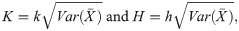
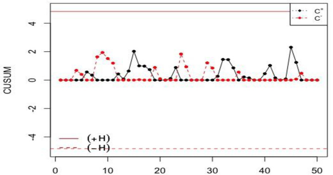
Application of the NCUSUM $\bar{X}$ chart using simulated data

In this section, the performance of the NCUSUM $\bar{X}$ chart is compared to one of the classical CUSUM $\bar{X}$ chart using simulated data. Fifty observations are generated using the neutrosophic normal distribution. The first twenty observations are generated by assuming that the process is statistically in-control and the next 30 observations are generated by assuming that the process has shifted with δ = 0.25. The simulated data along with n_N∈[3,5], k_N∈[0.4,0.5], h_N∈[4.887,5.894], σ_0N∈[1.00,1.00], and NARL₁∈[28.53,41.29], so the shift should be detected between the 28^th and 41^st samples. The results from the simulated data are displayed in Figs 1 and 2 for the proposed NCUSUM chart and the existing classical CUSUM $\bar{X}$ chart, respectively.

The proposed NCUSUM X¯ chart for simulated dataset.

Fig 1

The proposed NCUSUM $\bar{X}$ chart for simulated dataset.

The classical CUSUM X¯ chart for simulated dataset.

Fig 2

The classical CUSUM $\bar{X}$ chart for simulated dataset.

From Figs 1 and 2, it can be seen that the proposed NCUSUM $\bar{X}$ chart detects the first shift at around the 30^th sample in between the 28^th and 41^st samples; however, the classical CUSUM $\bar{X}$ chart indicates that all the charting statistics are in-control. Hence, it can be deduced that, the proposed NCUSUM $\bar{X}$ chart has the ability to detect the shifts in the process mean earlier as compared to its classical counterpart. Therefore, the NCUSUM $\bar{X}$ chart is more efficient and performs better than the classical CUSUM $\bar{X}$ chart.

Real-data application of the proposed CUSUM $\bar{X}$ chart

This section presents case-studies for the NCUSUM $\bar{X}$ chart that were applied to two types of data; the first example was dedicated to the case-study on the Pakistan state oil (PSO), while the second example is the case-study on the weather forecasting. The data were taken from the Stock Exchange and Meteorological Department of Pakistan. However, as mentioned in [28], all the observations and measurements of the current variables are not crisp numbers; they are neutrosophically varied with some indeterminacy in representing intervals instead of singleton numbers.

Petroleum industry case-study (PSO)

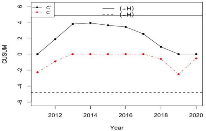
The oil prices are strongly related with the stock prices, which is dependent on the principle of demand and there are some indeterminacy in its measurements. The dataset in Table 8 denotes the stock price in 8 different days of August of the last 10 years for the PSO. For this data, let n_N = 8 and NARL₀ = 370. The reference value $K_{N} = {0.5 σ}_{0 N} / \sqrt{n_{N}}$ (i.e. k = 0.5), and decision interval $H_{N} = {h σ}_{0 N} / \sqrt{n_{N}}$ , where σ_0N∈[1.9221,2.239], n_N = 8 and h = 4.804 are determined by using the procedure used to derive the values in Tables 1–3. Thus, the calculated decision interval and reference value given in Eq (4) is H_N∈[3.265,3.803] and K_N∈[0.3397.0.3958]. The calculated charting statistics of the NCUSUM chart (i.e. $M_{N i}^{+}$ and $M_{N i}^{-}$ ) according to Eq (3) are provided in the last two columns of Table 8 and also plotted in Fig 3; however, those of the existing classical CUSUM $\bar{X}$ chart are plotted in Fig 4.

Real-life data from PSO petroleum oil company’s stock price for the proposed NCUSUM X¯ chart with HN∈[3.265, 3.803] and KN∈[0.3397, 0.3958].

Fig 3

Real-life data from PSO petroleum oil company’s stock price for the proposed NCUSUM $\bar{X}$ chart with H_N∈[3.265, 3.803] and K_N∈[0.3397, 0.3958].

Real-life data from PSO petroleum company’s stock price for the classical CUSUM X¯ chart with h = 4.804 and k = 0.5.

Fig 4

Real-life data from PSO petroleum company’s stock price for the classical CUSUM $\bar{X}$ chart with h = 4.804 and k = 0.5.

Table 8

Real-life example based on the PSO petroleum company’s stock price where h = 4.804, k = 0.5, n = 8, H_N∈[3.265, 3.803], μ_N∈[226.897, 232.9635] and σ_N∈[1.9221, 2.239].

	PSO petroleum oil company’s stock price
Year	AUGD10	AUGD11	AUGD12	AUGD13	AUGD17	AUGD18	AUGD19	AUGD20
2020	[182.00,185.25]	[184.6,190.00]	[184.01,190.52]	[182.9,185.75]	[185.51,197.00]	[191.5,197.00]	[190.51,194.75]	[190.0,194.99]	[186.37,191.90]	[0.00,0.00]	[-0.56,-0.54]
2019	[132.0,138.01]	[132.0,138.01]	[132.0,138.01]	[132.0,138.01]	[127.26,132.00]	[127.26,132.00]	[126.25,134.24]	[132.5,137.79]	[130.16,136.01]	[0.00,0.00]	[-2.62,-2.51]
2018	[279.17,283.24]	[279.17,283.24]	[279.17,283.24]	[288.71,294.62]	[284.57,290.25]	[284.57,290.25]	[284.57,290.25]	[283.33,292.08]	[282.91,288.39]	[0.91,0.97]	[-0.64,-0.60]
2017	[318.06,329.86]	[311.11,320.83]	[311.11,320.83]	[311.11,320.83]	[304.19,311.73]	[301.04,309.38]	[301.04,309.38]	[301.04,309.38]	[307.33,316.52]	[2.53,2.59]	[0.00,0.00]
2016	[286.46,290.90]	[285.08,287.50]	[285.08,288.19]	[285.08,288.19]	[284.03,288.19]	[281.25,284.73]	[279.52,283.82]	[279.52,283.82]	[283.25,286.91]	[3.40,3.57]	[0.00,0.00]
2015	[261.81,267.08]	[263.87,267.63]	[261.81,265.28]	[256.25,264.58]	[250.83,257.64]	[252.86,256.04]	[250.38,256.25]	[244.62,250.69]	[255.31,260.64]	[3.61,3.83]	[0.00,0.00]
2014	[265.69,269.79]	[253.67,267.02]	[247.58,256.24]	[248.73,259.73]	[254.31,263.67]	[258.86,268.48]	[254.25,261.81]	[254.86,263.53]	[254.74,263.77]	[3.89,4.06]	[0.00,0.00]
2013	[228.47,244.73]	[228.47,244.73]	[244.73,251.03]	[245.87,250.63]	[240.35,245.98]	[240.35,245.98]	[237.23,249.46]	[243.23,251.03]	[238.58,247.94]	[3.77,3.87]	[0.00,0.00]
2012	[175.14,177.57]	[175.14,177.57]	[175.14,177.57]	[175.00,180.56]	[174.79,176.39]	[174.79,176.39]	[174.79,176.39]	[174.79,176.39]	[174.94,177.35]	[1.86,2.00]	[-0.91,-0.87]
2011	[145.94,149.97]	[148.61,157.46]	[157.64,163.19]	[157.64,163.19]	[165.01,167.71]	[160.42,165.28]	[153.92,157.23]	[153.92,157.23]	[155.38,160.15]	[0.00,0.00]	[-2.27,-2.25]

From Fig 3, it can be noted that the PSO petroleum stock price are out-of-control in 2013 to 2015 (i.e. higher prices); while, in 2011 and 2012 the petroleum oil prices are in-control (within reasonable range). However, after 2015, the prices are decreasing and are in-control. From Fig 4, it can be seen that in all the monitored years, the PSO petroleum prices are in-control. From the comparison of both the charts, it can be seen that the proposed neutrosophic chart performs better and detects shifts earlier as compared to the classical counterpart.

Pakistan meteorological case-study

For the Meteorological Department dataset of Pakistan, the application of the proposed NCUSUM $\bar{X}$ chart is discussed. Since weather warning is a vital forecast because it is used for protecting people’s property and well-being as well as some socio-economic benefits. Thus, numerical weather experts use advanced mathematical formulas to predict the weather. Table 9 shows the weather forecast data information from 9 different cities in Pakistan for 12 months. The abbreviations symbols for the cities name are: Lahore = LHR, Karachi = KHI, Multan = MUX, Faisalabad = FSD, Islamabad = ISB, Peshawar = PEW, Hyderabad = HDD, Skardu = KDU and Gilgit = GIL.

Table 9

Meteorological department dataset for real-life example with design parameters h = 4.791, H = 1.409, k = 0.5 and n = 12.

	Weather Update by Month
City	Jan	Feb	Mar	April	May	Jun	July	Aug.	Sep.	Oct	Nov	Dec
LHR	[5.9,19.8]	[8.9,22.0]	[14.0,27.1]	[19.6,33.9]	[23.7,38.6]	[27.4,40.4]	[26.9,36.1]	[26.4,35.0]	[24.4,35.0]	[18.2,32.9]	[11.6,27.4]	[6.8,21.6]	[17.81,30.81]	[0.00,0.15]	[0.00,0.00]
KHI	[10.4,25.8]	[12.7,27.7]	[17.6,31.5]	[22.3,34.3]	[25.9,35.2]	[27.9,34.8]	[27.4,33.1]	[26.1,31.7]	[25.2,32.6]	[21,34.7]	[15.9,31.9]	[11.6,27.4]	[20.35,31.72]	[0.16,0.81]	[0.00,0.00]
MUX	[4.5,21]	[7.6,23.2]	[13.5,28.5]	[19.5,35.5]	[24.4,40.4]	[28.6,42.3]	[28.7,39.2]	[28,38]	[24.9,37.2]	[18.2,34.6]	[10.9,28.5]	[5.5,22.7]	[17.85,32.61]	[0.49,0.98]	[0.00,0.00]
FSD	[4.4,19.4]	[7.4,22.4]	[12.6,27.3]	[18.1,33.8]	[23.3,38.9]	[27.4,40.7]	[27.4,37.3]	[26.9,36.3]	[24.2,36]	[17.6,33.6]	[10.4,27.5]	[5.7,21.8]	[17.11,31.25]	[0.56,0.99]	[0.00,0.00]
ISB	[2.6,17.7]	[5.1,19.1]	[9.9,23.9]	[15,30.1]	[19.7,35.3]	[23.7,38.7]	[24.3,35]	[23.5,33.4]	[20.6,33.5]	[13.9,30.9]	[7.5,25.4]	[3.4,19.7]	[14.10,28.55]	[0.13,0.42]	[0.00,0.00]
PEW	[4,18.3]	[6.3,19.5]	[11.2,23.7]	[16.4,30]	[21.3,35.9]	[25.7,40.4]	[26.6,37.7]	[25.7,35.7]	[22.7,35]	[16.1,31.2]	[7.6,25.6]	[4.9,20.1]	[15.70,29.42]	[0.00,0.16]	[0.00,0.00]
HDD	[11.1,25]	[13.6,28.1]	[18.5,33.9]	[23,38.9]	[26.2,41.6]	[28.1,40.2]	[27.8,37.4]	[26.7,36.3]	[25.3,36.8]	[22.3,37.2]	[17.3,31.9]	[12.5,26.3]	[21.03,34.46]	[0.68,0.95]	[0.00,0.00]
KDU	[-12,-3]	[-11,-1]	[-5,5]	[0,12]	[3,15]	[7,20]	[10,23]	[10,22]	[5,20]	[-1,14]	[-6,7]	[-10,0]	[-0.83,11.16]	[0.00,0.00]	[-2.72,-2.52]
GIL	[-2.7,9.6]	[0.4,12.6]	[5.4,18.4]	[9.2,24.2]	[11.8,29]	[14.9,34.2]	[18.2,36.2]	[17.5,35.3]	[12.4,31.8]	[6.3,25.6]	[0.4,18.4]	[-2.3,11.6]	[7.62,23.91]	[0.00,0.00]	[-3.45,-3.02]

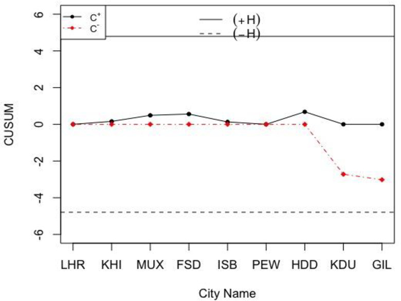
Let the sample size and the in-control ARL values be n_N = 12 and NARL₀ = 370, while the reference and decision interval values are H_N∈[1.4109,2.6919] and K_N∈[0.1472,0.2809] when h = 4.791, k = 0.5, and σ_0N∈[1.0197,1.9464]. So, the calculated NCUSUM charting statistics (i.e. $M_{N i}^{+}$ and $M_{N i}^{-}$ ) are given in the last two columns of Table 9. The charting statistics of the proposed NCUSUM $\bar{X}$ chart are shown in Fig 5 and the ones of the classical CUSUM $\bar{X}$ chart are shown in Fig 6.

The proposed NCUSUM X¯ chart for the weather condition in Pakistan with HN∈[1.4109, 2.6919] and KN∈[0.1472, 0.2809].

Fig 5

The proposed NCUSUM $\bar{X}$ chart for the weather condition in Pakistan with H_N∈[1.4109, 2.6919] and K_N∈[0.1472, 0.2809].

The classical CUSUM X¯ chart for the weather data with h = 4.791 and k = 0.5.

Fig 6

The classical CUSUM $\bar{X}$ chart for the weather data with h = 4.791 and k = 0.5.

From Fig 5, the proposed NCUSUM $\bar{X}$ chart is found to be more efficient and gives better results compared to its classical counterpart in Fig 6; as it indicates downwards shift in the weather forecast and shows that the weather is very cold in Skardu and Gilgit cities. Note though, the classical CUSUM $\bar{X}$ chart reveals that all cities’ weather are within normal range and does not detect the shift at any point in the data. Thus, in comparison of both the control charts for monitoring weather forecasting, we can say that the NCUSUM $\bar{X}$ chart provides better prediction especially when meteorologists are not sure about the temperature values to be used for weather prediction. Therefore, the neutrosophic CUSUM $\bar{X}$ chart is recommended for weather prediction under the uncertainty environments.

Conclusion and future recommendations

In this paper, a new NCUSUM $\bar{X}$ control chart is proposed. The neutrosophic run length performance of the proposed chart is computed using Monte Carlo simulations. The application of the proposed chart is illustrated using simulated data and two real-life examples using the PSO petroleum industry dataset and the weather forecasting dataset from nine cities in Pakistan. The results show that the NCUSUM $\bar{X}$ chart is better suited for use than the classical CUSUM $\bar{X}$ chart either when the data are inaccurate or when the operators do not have a complete dataset or for uncertain environments situations. The comparison study shows that the proposed neutrosophic chart is efficient in detecting small to large shifts in the process parameter than the classical chart. Note that the NCUSUM $\bar{X}$ chart is functional when the variable of interest adopts the neutrosophic normal distribution. The proposed neutrosophic chart is also recommended for monitoring the process mean shifts for the medical instruments, automobiles, aerospace and drinking water industries.

Further future works can be dedicated to the NCUSUM $\bar{X}$ chart that can be designed for non-normal distributions, as well as for the multiple dependent state sampling and repetitive sampling approaches.

Acknowledgements

The authors are deeply thankful to the editor and reviewers for their valuable suggestions to improve the quality of the original manuscript.

References

DCMontgomery, Introduction to Statistical Quality Control, 6th Edition, John Wiley & Sons, Hoboken, New Jersey; 2009.

JMLucas, MSSaccucci. Exponentially weighted moving average control schemes: Properties and enhancements. Technometrics. 1990; 32(1): 1–12. 10.1080/00401706.1990.10484583

YIZhao, FTsung, FWang. Dual CUSUM control schemes for detecting a range of mean shifts. IIE Transactions. 2005; 37(11): 1047–1057. 10.1080/07408170500232321.

ZLi, ZWang. Adaptive CUSUM of the Q chart. International Journal of Production Research. 2010; 48(5): 1287–1301. 10.1080/00207540802484937.

AShafqat, ZHuang, MAslam, and MSNawaz. A Nonparametric repetitive sampling DEWMA control chart based on linear prediction. IEEE Access; 2020; 8: 74977–74990. 10.1109/ACCESS.2020.2989132.

A.Haq An improved mean deviation exponentially weighted moving average control chart to monitor process dispersion under ranked set sampling. Journal of Statistical Computation and Simulation. 2014; 84(9), 2011–2024 10.1080/00949655.2013.780059

AHaq, JBrown, and EMoltchanova. New exponentially weighted moving average control charts for monitoring process mean and process dispersion. Quality and Reliability Engineering International. 2015; 31(5): 877–901. 10.1002/qre.1646.

AHaq, JBrown, EMoltchanova, AIAl-Omari. Effect of measurement error on exponentially weighted moving average control charts under ranked set sampling schemes. Journal of Statistical Computation and Simulation. 2015; 85(6): 1224–1246. 10.1080/00949655.2013.873040.

RASanusi, MRiaz, NAAdegoke, MXie. An EWMA monitoring scheme with a single auxiliary variable for industrial processes. Computers & Industrial Engineering. 2017; 114: 1–10. 10.1016/j.cie.2017.10.001.

AShafqat, ZHuang, MAslam. Design of X-bar control chart based on Inverse Rayleigh Distribution under repetitive group sampling. Ain Shams Engineering Journal. 2020; 10.1016/j.asej.2020.06.001.

A.Shafqat, J.Hussain, A. D.Al-Nasser, and M.Aslam Attribute control chart for some popular distributions. Communications in Statistics—Theory and Methods. 2018; 47(8):1978–1988. 10.1080/03610926.2017.1335414.

MKhademi, VAmirzadeh. Fuzzy rules for fuzzy x and r control charts. Iranian Journal of Fuzzy Systems., 2014; 11(5): 55–66. 10.22111/IJFS.2014.1722.

MHZSabegh, AMirzazadeh, SSalehian, GWWeber. A literature review on the fuzzy control chart: classifications & analysis. International Journal of Supply and Operations Management. 2014; 1(2): 167–189. 10.22034/2014.2.03.

SSenturk, NErginel. Development of fuzzy

\tilde{\bar{X}} ‐ \tilde{R}

and

\tilde{\bar{X}} ‐ \tilde{S}

control charts using α-cuts. Information Sciences. 2009; 179(10):1542–1551. 10.1016/j.ins.2008.09.022.

AFaraz, RBKazemzadeh, MBMoghadam, ABazdar. Constructing a fuzzy Shewhart control chart for variables when uncertainty and randomness are combined. Quality & Quantity, 2010; 44: 905–914. 10.1007/s11135-009-9244-9.

F.Smarandache Neutrosophic Logic—A generalization of the intuitionistic fuzzy logic. SSRN Electronic Journal, 2016 10.2139/ssrn.2721587.

F.Smarandache Introduction to Neutrosophic Statistics, Sitech & Education Publishing, Craiova, Romania & Ohio, USA; 2014.

HEKhalid, AKEssa. Introduction to Neutrosophic Statistics, the translated Arabic version, Pons Publishing House, Brussels, Belgium, 2020.

JCSMorán, JFEChuga, WMACollaguazo, CWMGudiño. Neutrosophic statistics applied to the analysis of socially responsible participation in the community. Neutrosophic Sets and Systems, 2019; 26:19–28. 10.5281/zenodo.3244232.

PACMaldonado, YPMartinez, GSEValverde, JDIErazo. Neutrosophic statistics methods applied to demonstrate the extra-contractual liability of the state from the Administrative Organic Code. Neutrosophic Sets and Systems, 2019; 26:29–34. 10.5281/zenodo.3244262.

RMCarballido, HParonyan, MAMatos, ALSMolina. Neutrosofic statistics applied to demonstrate the importance of humanistic and higher education components in students of legal careers. Neutrosophic Sets and Systems, 2019; 26:174–180. 10.5281/zenodo.3244848

CPanthong, APongpullponsak. Non-normality and the fuzzy theory for variable parameters

\bar{X}

control charts. Thai Journal of Mathematics, 2016; 14(1):203–213.

PPereira, JSeghatchian, BCaldeira, SXavier, Gde Sousa. Statistical methods to the control of the production of blood components: Principles and control charts for variables. Transfusion and Apheresis Science, 2018; 57(1):132–142. 10.1016/j.transci.2018.02.022

MAslam, RARBantan, NKhan. Design of a new attribute control chart under neutrosophic statistics. International Journal of Fuzzy Systems, 2019; 21:433–440. 10.1007/s40815-018-0577-1.

MAslam, GSRao, AShafqat, LAhmad, RAKSherwani. Monitoring circuit boards products in the presence of indeterminacy. Measurement, 2021; 168:108404 10.1016/j.measurement.2020.108404.

ZKhan, MGulistan, RHashim, NYaqoob, WChammam. Design of S-control chart for neutrosophic data: An application to manufacturing industry. Journal of Intelligent & Fuzzy Systems. 2020; 38(4): 4743–4751. 10.3233/JIFS-191439.

M.Aslam Attribute Control Chart Using the Repetitive Sampling under Neutrosophic System. IEEE Access, 2019; 7:15367–15374. 10.1109/ACCESS.2019.2895162.

M.Aslam Control chart for variance using repetitive sampling under neutrosophic statistical interval system. IEEE Access, 2019; 7: 25253–25262. 10.1109/ACCESS.2019.2899020.

ESPage. Continuous inspection schemes. Biometrika, 1954; 41(1–2): 100–115. 10.1093/biomet/41.1-2.100.

Introduction

The CUSUM control chart

The classical CUSUM chart

The proposed neutrosophic CUSUM chart

Run length performance

Performance of the NCUSUM X¯ chart

Comparison of the proposed NCUSUM X¯ and classical CUSUM X¯ charts

Application of the NCUSUM X¯ chart using simulated data

Real-data application of the proposed CUSUM X¯ chart

Petroleum industry case-study (PSO)

Pakistan meteorological case-study

Conclusion and future recommendations

Acknowledgements

References

Performance of the NCUSUM $\bar{X}$ chart

Comparison of the proposed NCUSUM $\bar{X}$ and classical CUSUM $\bar{X}$ charts

Application of the NCUSUM $\bar{X}$ chart using simulated data

Real-data application of the proposed CUSUM $\bar{X}$ chart