 Exact solutions for the 2d-strip packing problem using the positions-and-covering methodology
PLoS ONE


Competing Interests: The authors have declared that no competing interests exist.

- Altmetric
We use the Positions and Covering methodology to obtain exact solutions for the two-dimensional, non-guillotine restricted, strip packing problem. In this classical NP-hard problem, a given set of rectangular items has to be packed into a strip of fixed weight and infinite height. The objective consists in determining the minimum height of the strip. The Positions and Covering methodology is based on a two-stage procedure. First, it is generated, in a pseudo-polynomial way, a set of valid positions in which an item can be packed into the strip. Then, by using a set-covering formulation, the best configuration of items into the strip is selected. Based on the literature benchmark, experimental results validate the quality of the solutions and method’s effectiveness for small and medium-size instances. To the best of our knowledge, this is the first approach that generates optimal solutions for some literature instances for which the optimal solution was unknown before this study.
Introduction
The Two-Dimensional Strip Packing Problem (2SP) is composed of a given set of n rectangular items, each one with specific width wi and height hi, for i = 1, …, n, and a strip of width W and infinite height. The aim is to place all the items into the strip orthogonally; without overlapping, minimizing the overall strip’s height [1, 2]. We assume that all input data wi, hi, and W are positive integers and that wi ≤ W for all items i = 1, …, n. We consider the case when the items have a fixed orientation, and the guillotine cut constraint is unnecessary.
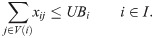
The 2SP is NP-hard in the strong sense since it can be reduced to the one-dimensional bin-packing problem [2–4], and according to the typology proposed by [5], the 2SP belongs to the class of cutting and packing problems: two-dimensional, open dimension problem (2D-ODP). Fig 1 shows the optimal configuration for an instance proposed by [6] with 50 items and a strip of width W = 40. The optimal height is H = 15. In this case, there is no wasting in the strip; that is, we have a perfect packing.

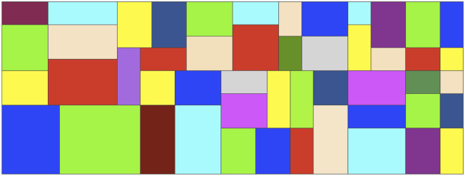
Example for 2SP.
The optimal configuration for an instance proposed by [6] with 50 items, a strip of width W = 40, and an optimal height H = 15.
Many real-world applications of this problem can be found in the paper, textile, glass, steel, and wood industries, where rectangular items are cut from larger rectangular sheets of material that can be considered with infinite height [7, 8]. The 2SP also appears in scheduling problems where the tasks require a contiguous subset of identical resources [9].
In this study, we propose an adaptation of the Positions and Covering (P&C) methodology, used by [10] to obtain optimal solutions for the two-dimensional bin packing problem. Considering the similarity of the 2SP with other packing problems, some potential applications for the P&C methodology can be found in agricultural fields to delineate rectangular and homogeneous management zones [11–13], in scheduling problems applied to environmental, automotive, ferry, and manufacturing industries to ensure maximum use of materials [14–16], in healthcare applied to operating rooms schedules [17–19], in cloud computing where a set of jobs must be processed on virtual machines of physical servers with the aim of improves the energy efficiency [20–22], and in optimal deliveries in e-commerce where the objective is optimizing the total number of containers to integrate into several delivery trips [23].
The P&C methodology adapted to the 2SP is as follows. Given an instance of the 2SP, the first step of the P&C is to compute the strip’s height with the assumption that a perfect packing exists. Then we generated a set of valid positions to determine all possible places to locate it on the strip for each item. This pre-processing is the key-point of the P&C methodology. Finally, using the H computed, the P&C solves a set-covering model for the decision version of the 2SP (D-2SP(H)): is there a non-overlapping packing of the n items into the strip with H height? If there is a feasible solution, then H is the optimal value for the 2SP. Otherwise, P&C iterates again, increasing the height H of the strip by one. The P&C is an exact methodology that obtains optimal solutions for the 2SP, that is, every time our methodology is executed, the same solution and time are going to be obtained.
The main differences of our methodology with respect to the mentioned exact approaches is that the P&C groups the items with identical size and computes their demand. Indeed, all the other approaches consider similar items as individual. This grouping makes a better covering model that can be solved faster. Moreover, this new set-covering formulation is strengthened with two families of valid inequalities. This manner, the P&C methodology is power enough to obtain optimal solutions for the 2SP problem without any more complex methodology as column generation.
Because of the combinatorial complexity of the 2SP, the attempts to solve it are roughly divided into exact and approximation methods. Some reviews of the 2SP are presented in [8, 24, 25], and some surveys for packing and cutting problems are showed in [26–29].
In terms of other exact methods, there have been recent combinatorial branch-and-bound (B&B) algorithms that build solutions by packing items one at a time in the strip like the ones of [1, 2, 30–33]. In [1], the authors propose a B&B algorithm to solve the 2D rectangular packing problems, a particular case of the 2SP. This B&B algorithm is enhanced with a dynamic programming mechanism for determining if gaps can be filled.
A new relaxation to produce good lower bounds and obtain practical heuristic algorithms is introduced in [2]. These bounds were also used in a B&B algorithm. The authors of [33] propose two algorithms for the 2SP with and without 90-degrees rotations. They are based on a branching operation that uses the staircase placement. Two exact algorithms and an approximate algorithm have been proposed by [34] to solve a variant of the strip cutting problem. These algorithms are based on B&B and dynamic programming procedures.
Concerning the heuristics and metaheuristics methods to solve the 2SP, in [3], the authors introduce the bottom-left (BL) heuristic. Some approaches with variants or implementations of the BL strategy to solve packing problems can be found in [6, 35–39]. Other works that implement metaheuristics methods as tabu-search, simulated annealing, and genetic algorithms are presented in [40–43].
In [44], the authors propose two metaheuristics that involve the application of the simulated annealing with a heuristic construction algorithm. In many of these studies, the authors use a version of the BL heuristic to arrange the items. In [45] the authors show some models strengthen with well-known valid inequalities and based on the work of [43]. Some improvements for the best-fist heuristic, where it is presented a simple local random local search, are showed in the work of [46]. The use of data mining techniques also has been implemented to assess the quality of heuristics solutions [47]. Other approaches that consider hierarchical or multi-stage methodologies can be found in the works of [48–50]. A survey of heuristics for the two-dimensional rectangular strip packing problem is presented in [51], and upper bounds for heuristic approaches in [52].
The main strength of the P&C methodology for the 2SP is that it obtains optimal solutions for many instances of the classical benchmarks that none of the previous (and more elaborated) methods could find. For example, the P&C solved to optimality several instances proposed by [53] for which the optimal solutions were not known before of this study. To the best of our knowledge, the P&C methodology is one of the best methods to find optimal solutions for the 2SP for small and medium-size instances.
The rest of this article is organized as follows. In Section Materials and methods, we describe the P&C methodology for the 2SP. In Section Results, we present the experimental results for the P&C methodology by using a set of small and medium-size instances that have been broadly used in the literature to test other algorithms. Finally, in Section Conclusions, we make some concluding remarks.
Materials and methods
In this section, we present the materials and methods used to solve the 2SP. First, we show the adaptation of the P&C proposed by [10] to solve the 2d-bin packing problem. Then, we describe each part of the methodology for the 2SP.
The P&C methodology for the 2SP
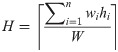
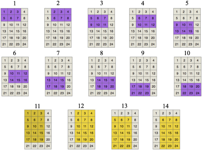
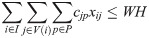
The adaptation of the P&C methodology for the 2SP is schematized in Fig 2. Given an instance of the 2SP, the first step is to compute the height H of the strip, assuming that a perfect packing exists, that is, the total area of the items divided by the width of the strip, as shown in Eq (1). Notice that if a better lower bound of the 2SP instance is known, then this first value of the height could be updated, and some iterations of the P&C may be avoided.
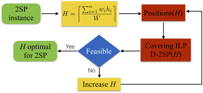
Adaptation of the P&C methodology.
The two-step methodology to solve the 2SP.
Considering this H-value, the P&C generates the set of valid positions that locate the items inside of the strip. This step is the key-point of our methodology, and it will be later explained in detail. Then, an integer linear programming set-covering formulation (ILP) for the decision version of the 2SP, named as D-2SP(H), is solved to optimality. If the covering model is feasible, then H is the optimal height of the strip. Else, the H-value is increased by one or in a dichotomous way, the new set of valid positions for the items is generated, and the covering model is solved again. These last three steps represent the main difference with the P&C for the 2D-BPP (see [10]). The procedure ends when P&C finds a feasible solution of the D-2SP(H), and the current height becomes the optimal one.
Positions stage for the 2SP
The objective of the Positions stage is to generate the set of valid positions where an item can be placed into the strip, that is, from the infinite set of positions that an item can take in the bin, the P&C determines only a finite set that guarantees the optimality of the solution. The inputs of the Positions stage are i) the number n of items with their specifics width wi, height hi, and demand di, ii) the width W of the strip, and iii) the current height H of the strip (first computed with Eq 1 or a known lower bound, or an updated value).
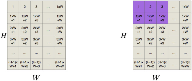
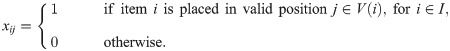
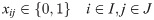
With the current height H of the strip, the first step in the Positions stage is to delineate a Cartesian grid inside the strip, that is, a regular tessellation of the 2-dimensional Euclidean space by congruent unit squares, where each square has a particular identification. We arbitrarily choose the enumeration that starts at the top left corner square and ends at the bottom right square (see Fig 3a). Thus, for each item, a valid position is created if its top left corner coincides with a tiling, and its width and height dimensions do not exceed the size of the strip. Each valid position is labeled to differentiate one from each other. Fig 3b shows the valid position for an item with dimensions 2 × 3 with its top-left corner at tile 1. Notice that the position which starts in the tile 1 × W would not be a valid position for this item. Let JH be the set of valid positions for all the items for a fixed height H of the strip. To generate JH, we start populating its valid positions width-wise and then length-wise for each item. The size of JH is pseudo-polynomial, but this pre-processing allows the P&C method to decompose the problem and to reach optimal solutions.
First step of the P&C methodology.
a) Grid inside of the strip and b) Valid position for an item with dimensions 2 × 3 with its top-left corner at tile 1.
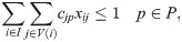
Fig 4 shows the set of valid positions for an item of 2 × 3 and an item of 5 × 3 in a strip with dimensions 6 × 4. In this case, JH has 14 valid positions. The set from 1 to 10 corresponds for the first item while the set from 11 to 14 to the second item. Each valid position is unique; therefore, it has a specific label and an unrepeatable tiles set. For example, position 1 (corresponding to the 2 × 3 item) contains tiles 1, 2, 3, 5, 6, and 7.
Generation of positions.
Set JH of valid positions for items of 2 × 3 and 5 × 3 in a strip with H = 6 and W = 4.
The resulting set of valid positions may be view as a correspondence matrix CH = {cjp}, where rows represent the set of valid positions j ∈ JH and columns are the tiles in the strip. Matrix CH is composed of 1’s and 0’s, where cjp = 1 if valid position j covers tile p, cjp = 0 otherwise. The correspondence matrix of Fig 4 (set JH for an item of 2 × 3 and another one of 5 × 3 in a strip with H = 6 and W = 4) appears in Table 1. Each row in the correspondence matrix represents the respective valid position presented in Fig 4. For example, row 1 has ones in tiles 1, 2, 3, 5, 6, and 7, which correspond with position 1 of the figure.

| Tiles on the strip (p) | |||||||||||||||||
|---|---|---|---|---|---|---|---|---|---|---|---|---|---|---|---|---|---|
| 1 | 2 | 3 | 4 | 5 | 6 | 7 | 8 | 9 | 10 | 11 | 12 | 13 | 14 | … | 24 | ||
| Valid positions (j) | 1 | 1 | 1 | 1 | 0 | 1 | 1 | 1 | 0 | 0 | 0 | 0 | 0 | 0 | 0 | … | 0 |
| 2 | 0 | 1 | 1 | 1 | 0 | 1 | 1 | 1 | 0 | 0 | 0 | 0 | 0 | 0 | … | 0 | |
| 3 | 0 | 0 | 0 | 0 | 1 | 1 | 1 | 0 | 1 | 1 | 1 | 0 | 0 | 0 | … | 0 | |
| 4 | 0 | 0 | 0 | 0 | 0 | 1 | 1 | 1 | 0 | 1 | 1 | 1 | 0 | 0 | … | 0 | |
| 5 | 0 | 0 | 0 | 0 | 0 | 0 | 0 | 0 | 1 | 1 | 1 | 0 | 1 | 1 | … | 0 | |
| 6 | 0 | 0 | 0 | 0 | 0 | 0 | 0 | 0 | 0 | 1 | 1 | 1 | 0 | 1 | … | 0 | |
| 7 | 0 | 0 | 0 | 0 | 0 | 0 | 0 | 0 | 0 | 0 | 0 | 0 | 1 | 1 | … | 0 | |
| 8 | 0 | 0 | 0 | 0 | 0 | 0 | 0 | 0 | 0 | 0 | 0 | 0 | 0 | 1 | … | 0 | |
| 9 | 0 | 0 | 0 | 0 | 0 | 0 | 0 | 0 | 0 | 0 | 0 | 0 | 0 | 0 | … | 0 | |
| 10 | 0 | 0 | 0 | 0 | 0 | 0 | 0 | 0 | 0 | 0 | 0 | 0 | 0 | 0 | … | 1 | |
| 11 | 1 | 1 | 1 | 0 | 1 | 1 | 1 | 0 | 1 | 1 | 1 | 0 | 1 | 1 | … | 0 | |
| 12 | 0 | 1 | 1 | 1 | 0 | 1 | 1 | 1 | 0 | 1 | 1 | 1 | 0 | 1 | … | 0 | |
| 13 | 0 | 0 | 0 | 0 | 1 | 1 | 1 | 0 | 1 | 1 | 1 | 0 | 1 | 1 | … | 0 | |
| 14 | 0 | 0 | 0 | 0 | 0 | 1 | 1 | 1 | 0 | 1 | 1 | 1 | 0 | 1 | … | 1 | |
Notice that the set of valid positions determined by the unitary grid is sufficient to reach the optimal solution of the 2SP since all input data are integer.
Covering stage
In this stage, the P&C executes a set-covering formulation based on an integer linear programming model. This formulation solves the decision problem for the strip packing problem D-2SP(H), that is, is there a solution for the 2SP when the height is set to H? If the answer is positive, then the procedure ends (since we are minimizing the height), else the height of the strip is increased by one. A new iteration begins by populating the new set of valid positions for each item, and the decision model is solved again.
Formalizing, let I be the set of items, recall that JH is the set of valid positions for a fixed height of the strip, V(i) be the subset of valid positions for each item i ∈ I where V(i)∈J, and P be the tiles set inside of the strip. Furthermore, we know other parameters such as the demand di of item i ∈ I and the maximum of times that this item can be packed inside the strip: UBi.
The decision variables for the ILP model are:
This manner, the set-covering formulation to solve the decision problem D-2SP(H) is as follows.

s.t.
Besides valid inequalities (5) and (6), other valid inequalities could enhance the ILP, but these proved in preliminary results to be the more efficient for the 2SP (and also for the 2BPP, see [10]).
Results
To test the P&C methodology, we use two sets of instances: the original benchmark for the strip packing and the benchmark for other two-dimensional cutting problems. The description for each group of instances is given in the following sections. Then, we present the experimental results on these sets.
Original instances for the strip packing
This instance set refers to the instances generated for the two-dimensional strip packing problem. This set contains:
2 perfect packing instances proposed by [6], known as jack01-jack02.
1 instance proposed by [56], known as kendall.
25 instances proposed by [34], known as hifi01-hifi25.
9 of 21 instances proposed by [36], known as hopper.
The optimum for instances dagli01, dagli03 and, dagli04 was not known until now, according to the Working Group on Cutting and Packing within the Association of the European Operational Research Societies (ESICUP) (https://www.euro-online.org/websites/esicup/data-sets/#1535972088188-55fb7640-4228).
For some instances like the hopper ones, we are no testing all of the instances of the benchmark since they are too large for the P&C methodology. Indeed, other instances benchmark exist in the literature but they are also too large for the P&C so they are not mentioned in this section.
Instances for other two-dimensional cutting problems
This set of instances was originally introduced for other two-dimensional cutting problems and was transformed into strip packing instances considering the item size and the bin width. We found the following instances:
100 of 300 instances proposed by [57]. These instances are divided into 10 classes (6 and 4, respectively), where each class is composed of 5 groups of 10 instances. Each group has a different number of items to be packed into the bin with n = {20, 40, 60, 80, 100}. The corresponding best-known solution and lower bound for each instance are available at http://www.or.deis.unibo.it/research_pages/ORinstances/2BP.html. This set of instances is known as the BW instances.
3 instances proposed by [58], known as cgcut.
12 instances proposed by [59], known as ngcut. The cgcut and ngcut instances are test problems for 2D cutting problems, which were transformed to 2D bin packing instances according to [60]. These instances are available from the ORLIB library.
10 instances generated by [61], known as beng. They are vailable at PackLib2 ([62]), http://www.ibr.cs.tu-bs.de/alg/packlib/index.shtml.
6 instances proposed by [33], known as kenmochi.
As in the original instances for the strip packing problem, there are other set of instances that we do not include in this study since they are too large for the P&C.
Computational results
To solve the set-covering formulation, we use the integer linear programming solver (B&B) of CPLEX 12.7 using its default options, except for the optimality parameter set to 0%. All the instances were executed on a computer equipped with a processor 8-Core Intel Xeon E5-2609 @1.70 GHz, and 64 GB of RAM. The time limit for the B&B execution was fixed to 8 hours (28800 seconds).
For all of the instances, we start the P&C methodology using the height of the strip H given by the best lower bound obtained in the literature. When this bound is not available, we compute the H parameter assuming that a perfect packing exists (Eq (1)). We report the execution time for the last iteration of the P&C.
We compare the P&C with several methodologies that were implemented and tested on computers with different characteristics. Thus, our comparison is informative more than comparative. The main purpose of this study is to obtain optimal solutions for instances of the 2SP. Furthermore, statistical tests are not required to determine the solution quality because P&C is an exact method without statistical components on its procedure.
Original instances for the strip packing
Tables 2–5 show the experimental results for the original instances of the 2SP. The structure of these tables is as follows: the first three columns describe the instance, that is, the name (“Inst”), the width size W of the strip, and the number n of items. The fourth column indicates the optimum (“Opt”) or the best lower bound known (“LB”) in the literature. Columns 5–7 present the values for the P&C methodology: the generation time in seconds of the correspondence matrix (“GT”), the execution time in seconds required by the B&B solver (“ET”), and the optimum value z*. In the last columns, we present the solutions obtained by other approaches in the literature.
| Inst | Size | Opt | P&C | Jakobs | Liu and Teng | Mumford–Valenzuela | Bortfeldt | |||
|---|---|---|---|---|---|---|---|---|---|---|
| W | n | GT | ET | z* | ||||||
| jack01 | 40 | 25 | 15 | 0.59 | 22.40 | 15 | 17 | 16 | 16 | 16 |
| jack02 | 40 | 50 | 15 | 0.71 | 14.70 | 15 | 17 | 16 | 16 | 15 |
| kendall | 80 | 13 | 140 | 65.70 | 1.59 | 140 | ||||
| Number of optimal solutions | 3/3 | 0/3 | 0/3 | 0/3 | 1/3 | |||||
| Inst | Size | LB | P&C | Ratanapan and Dagli | Dagli and Poshyanonda | Bortfeldt | |||||
|---|---|---|---|---|---|---|---|---|---|---|---|
| W | n | GT | ET | z* | % | ||||||
| dagli01 | 60 | 31 | 45 | 4.21 | 843.86 | 46 | 100 | 91.88 | – | 95.67 | |
| dagli02 | 60 | 21 | 40 | 1.87 | 4.41 | 40 | 100 | 92.50 | – | 97.56 | |
| dagli03 | 30 | 37 | 112 | 8.02 | 78.78 | 112 | 100 | 94.41 | 96.03 | 98.58 | |
| dagli04 | 20 | 37 | 161 | 10.43 | 17.89 | 209 | 100 | 208 | – | 97.15 | 97.62 |
| Number of optimal solutions | 3/4 | 0/4 | 0/4 | 0/4 | |||||||
A “-” mark means that the authors did not solve this particular instance.
| Inst | Size | LB | P&C | Hifi | Sbb | Sda | Sbp | |||||||
|---|---|---|---|---|---|---|---|---|---|---|---|---|---|---|
| W | n | GT | ET | z* | z | ET | z | ET | z | ET | z | ET | ||
| hifi01 | 5 | 10 | 13 | 0.01 | 0.00 | 13 | 13 | <0.10 | 13 | 0.00 | 13 | 0.00 | 13 | 0.00 |
| hifi02 | 4 | 11 | 40 | 0.01 | 0.08 | 40 | 40 | 0.30 | 40 | 0.00 | 40 | 0.00 | 40 | 0.00 |
| hifi03 | 6 | 15 | 14 | 0.01 | 0.06 | 14 | 14 | 0.30 | 14 | 7.10 | 14 | 403.83 | 19 | 0.00 |
| hifi04 | 6 | 11 | 19 | 0.01 | 0.02 | 20 | 20 | 0.60 | 20 | 2.45 | 20 | 160.35 | 22 | OM |
| hifi05 | 20 | 8 | 20 | 0.04 | 0.00 | 20 | 20 | 0.50 | 20 | 0.00 | 20 | 0.00 | 20 | 0.00 |
| hifi06 | 30 | 7 | 38 | 0.58 | 0.01 | 38 | 38 | 4.90 | 38 | 0.00 | 38 | 0.00 | 38 | 0.00 |
| hifi07 | 15 | 8 | 14 | 0.01 | 0.02 | 14 | 14 | 0.30 | 14 | 0.01 | 14 | 0.06 | 14 | 1.01 |
| hifi08 | 15 | 12 | 17 | 0.02 | 0.05 | 17 | 17 | 0.50 | 17 | 1.57 | 17 | 10.45 | 17 | 0.00 |
| hifi09 | 27 | 12 | 68 | 1.2 | 4.14 | 68 | 68 | 7.60 | 68 | 0.14 | 68 | 0.01 | 68 | 0.00 |
| hifi10 | 50 | 8 | 80 | 3.72 | 20.84 | 80 | 80 | 0.30 | 80 | 0.18 | 80 | 0.01 | 80 | 0.00 |
| hifi11 | 27 | 10 | 48 | 1.05 | 3.21 | 48 | 48 | 8.60 | 48 | 4.89 | 48 | 0.42 | 48 | 0.00 |
| hifi12 | 81 | 18 | 34 | 3.36 | 0.03 | 34 | 34 | 2.80 | 38 | 3600 | 34 | 0.01 | 38 | 3600 |
| hifi13 | 70 | 7 | 50 | 4.78 | 11.47 | 50 | 50 | 6.10 | 50 | 0.38 | 50 | 0.15 | 50 | 0.00 |
| hifi14 | 100 | 10 | 60 | 12.31 | 77.63 | 69 | 69 | 4.10 | 69 | 15.57 | 69 | 196.65 | 69 | 0.00 |
| hifi15 | 45 | 14 | 34 | 1.70 | 13.22 | 34 | 34 | 6.00 | 34 | 2688.13 | 34 | 445.94 | 34 | 0.00 |
| hifi16 | 6 | 14 | 32 | 0.02 | 0.11 | 33 | 33 | 1.40 | 33 | 606.12 | 33 | 216.83 | 35 | OM |
| hifi17 | 42 | 9 | 34 | 1.12 | 5.70 | 34 | 39 | 7.10 | 34 | 2.07 | 34 | 0.00 | 34 | 0.00 |
| hifi18 | 70 | 10 | 89 | 17.38 | 2777.12 | 100 | 101 | 10.70 | 100 | 9.43 | 100 | 97.03 | 100 | 88.25 |
| hifi19 | 5 | 12 | 25 | 0.01 | 0.08 | 25 | 26 | 0.30 | 26 | 0.01 | 26 | 16.36 | 27 | OM |
| hifi20 | 15 | 10 | 19 | 0.05 | 0.29 | 20 | 21 | 1.80 | 20 | 1.73 | 20 | 1.32 | 20 | 0.00 |
| hifi21 | 30 | 11 | 140 | 7.22 | 141.44 | 140 | 145 | 3.90 | 140 | 24.31 | 140 | 63.29 | 140 | 0.00 |
| hifi22 | 90 | 22 | 34 | 6.70 | 35.57 | 34 | 34 | 11.80 | 42 | 3600 | 39 | 1597.91 | 43 | 3600 |
| hifi23 | 15 | 12 | 34 | 0.08 | 0.21 | 34 | 35 | 1.50 | 34 | 37.97 | 34 | 24.07 | 39 | 0.00 |
| hifi24 | 50 | 10 | 103 | 18.96 | 995.92 | 109 | 114 | 18.90 | 109 | 19.34 | 109 | 71.05 | 109 | 0.00 |
| hifi25 | 25 | 15 | 35 | 0.82 | 14.04 | 35 | 36 | 11.50 | 36 | 3600 | 36 | 657.15 | 43 | 3600 |
| Number of optimal solutions | 25/25 | 17/25 | 21/25 | 22/25 | 15/25 | |||||||||
| Class | Inst | Size | Opt | P&C | Iori | Best-fit | Burke | Bortfeldt | GRASP | |||||||
|---|---|---|---|---|---|---|---|---|---|---|---|---|---|---|---|---|
| W | n | GT | ET | z* | BF+TS | BF+SA | BF+GA | Avg | Best | Avg | Best | |||||
| C1 | 01 | 20 | 16 | 20 | 0.21 | 0.00 | 20 | 20 | 21 | 20 | 20 | 20 | 20 | 20 | ||
| 02 | 20 | 17 | 20 | 0.20 | 12.67 | 20 | 21 | 22 | 21 | 20 | 21 | 20 | 20 | |||
| 03 | 20 | 16 | 20 | 0.19 | 2.42 | 20 | 20 | 24 | 20 | 20 | 20 | 20 | 20 | |||
| Average percentage deviation from optimum | 0 | 1.59 | 10.17 | 1.59 | 0 | 1.59 | 1.59 | 1.59 | 0 | 0 | ||||||
| C2 | 04 | 40 | 25 | 15 | 0.73 | 26.05 | 15 | 15 | 16 | 16 | 16 | 16 | 15 | 15 | ||
| 05 | 40 | 25 | 15 | 0.69 | 64.59 | 15 | 16 | 16 | 16 | 16 | 16 | 15 | 15 | |||
| 06 | 40 | 25 | 15 | 0.66 | 16.39 | 15 | 15 | 16 | 16 | 16 | 16 | 15 | 15 | |||
| Average percentage deviation from optimum | 0 | 2.08 | 6.25 | 6.25 | 6.25 | 6.25 | 3.33 | 2.08 | 0 | 0 | ||||||
| C3 | 07 | 60 | 28 | 30 | 7.58 | 2134.92 | 30 | 31 | 32 | 31 | 31 | 31 | 30 | 30 | ||
| 08 | 60 | 29 | 30 | 8.16 | 4334.20 | 30 | 31 | 34 | 32 | 31 | 32 | 31 | 31 | |||
| 09 | 60 | 28 | 30 | 8.02 | 0.05 | 30 | 30 | 33 | 31 | 31 | 31 | 30 | 30 | |||
| Average percentage deviation from optimum | 0 | 2.15 | 9.04 | 4.23 | 3.23 | 4.23 | 3.16 | 3.16 | 1.08 | 1.08 | ||||||
| Number of optimal solutions | 9/9 | 5/9 | 0/9 | 2/9 | 3/9 | 2/9 | 8/9 | 8/9 | ||||||||
The results for jack and kendall instances from [6] and [56] are showed in Table 2. The last four columns are the solutions obtained by other approaches such as the genetic algorithm combined with a deterministic algorithm proposed by Jakobs in [6], a bottom-left algorithm for the genetic algorithm proposed by Liu and Teng in [39], the genetic algorithm proposed by Mumford-Valenzuela in [63], and the genetic algorithm based on layouts proposed by Bortfeld in [41]. These approaches are heuristics, and no execution times were reported. To the best of our knowledge, there are no other exact algorithms that have solved these instances. The P&C is the only method that guarantees the optimal solution (bold numbers) for the three instances, which were solved in less than 70 seconds, considering the generation time of the correspondence matrix and the execution time of the B&B.
Table 3 shows the experimental results for dagli instances. For these instances, we add two columns for the P&C: column “%” represents the packing density which is added to make a comparison with the other approaches, and column “” that shows the best lower bound found by the P&C methodology when an instance is not solved to optimality considering the time limit. The last three columns show the results in terms of the average of packing density for other approaches (no execution times were reported for these algorithms) such as an object-based evolutionary algorithm proposed by Ratanapan and Dagli in [54, 55], an artificial neural network, mathematical programming and genetic algorithm proposed by Dagli and Poshyanonda in [53] and [64], and a genetic algorithm based on layouts proposed by Bortfeld in [41] (we report the best solution obtained by this author). The P&C improves or certifies the optimality of the lower bound in the literature for the four instances. The optimum for dagli01 and dagli03 was not known before of this study according to the Working Group on Cutting and Packing within EURO of the Association of the European Operational Research Societies (ESICUP). The P&C methodology was able to solve 3 of 4 instances to optimality obtaining the best average packings. Furthermore, the P&C improves the LB of the literature for dagli04 instance from 161 to 208. For this instance, our methodology cannot guarantee the optimality because the B&B reaches the time limit with the value of 208. However, it obtains a feasible packing for the value 209 and infeasible for 207. When the lower bound is not close to the optimum, as for dagli04, we searched for the optimal height of the strip in a dichotomous way. Notice that the times of the last iteration of the P&C methodology are less than 15 minutes.
The experimental results for hifi instances proposed by [34] are shown in Table 4. This table is interesting since it compares several dichotomous algorithms based on exact methodologies. The P&C is compared with four approaches of the literature (the last eight columns) such as the dichotomous exact approach based on a B&B and dynamic-programming procedures developed by Hifi in [34], the B&B algorithm of [65] called Sbb, based on the B&B of [2], the dichotomous algorithm of [65] named Sda, based on the one of [34] with the decision version problem solved with the model of [66], and the branch-and-price algorithm of [65] called Sbp. For each approach, we present its solution z and the execution time ET. Hifi’s algorithm was coded in C and tested on a Sparc-Server20 (module 712 MP). The Sbb, Sda and Sbp algorithms were coded in C++ and tested on a Pentium M 1.7 GHz with 1G of RAM. The column generation and linear programs were solved with CPLEX and Concert Technology.
For hifi instances, we are not comparing the dichotomous behavior that seems to be a promising characteristic for the 2SP, but, we are analyzing the exact algorithms that solve the one-dimensional problem. Indeed, the best algorithms in terms of solution value are P&C, Sda, and Sbb, respectively. To the best of our knowledge, the P&C methodology is the only one finding the optimal solution for instances hifi19 and hifi25. Furthermore, the execution times of the last iteration for the P&C are efficient since they are less than 45 minutes in the worst case (instance hifi18). Nevertheless, the execution times of Hifi’s algorithm seem more competitive.
The experimental results for small-medium size instances proposed by Hopper and Turton in [36] are presented in Table 5. We add a new column at the beginning of the table to specify the class of the instance. We compare the results of the P&C with the hybrid algorithm proposed in [42] (column 9). Columns 10–13 show the results obtained by the best-fit algorithm from [67] and its enhancements adding Tabu-search (TS), simulated-annealing (SA), and a genetic algorithm (GA) from [68]. In columns 14 and 15 are presented the average and best solutions obtained by the genetic algorithm presented in [41], the authors do not present detailed solutions for each instance. Finally, the last two columns show the average and best results obtained by the GRASP proposed by [40]. Numbers in bold represent the optimal solutions. To make a comparison of our methodology with respect to other approaches, we use the average percentage deviation from optimum proposed by [40]. This average is calculated as (sol–opt)/opt. The results show that the P&C algorithm obtains the best solutions for the first three classes (small-medium instances), getting 9 of 9 optimal solutions, improving the best results of the GRASP proposed by [40]. We do not present the results for large instances since P&C cannot obtain their optimal solutions. Indeed, the size of the correspondence matrix for these instances is too large, and the memory of our computer is not enough to solve them.
Instances for other two-dimensional cutting problems
In this section, we present the experimental results for the other two-dimensional cutting instances which have been adapted to the 2SP (Tables 6–10). The format for each table is similar to the previous ones.
| Inst | Size | Opt | P&C | Best fit | Burke | GRASP | |||||||
|---|---|---|---|---|---|---|---|---|---|---|---|---|---|
| W | n | GT | ET | z* | BF+TS | BF+SA | BF+GA | Average | Best | ||||
| N1 | 40 | 10 | 40 | 1.66 | 3.01 | 40 | 45 | 40 | 40 | 40 | 40 | 40 | |
| N2 | 30 | 20 | 50 | 2.98 | 72.64 | 50 | 53 | 50 | 50 | 50 | 50 | 50 | |
| N3 | 40 | 30 | 50 | 8.31 | 27.91 | 50 | 52 | 51 | 51 | 52 | 51 | 51 | |
| N4 | 80 | 40 | 80 | 102.85 | 25047.90 | 80 | 86 | 83 | 82 | 83 | 81 | 81 | |
| Number of optimal solutions | 4/4 | 0/4 | 2/4 | 2/4 | 2/4 | 2/4 | 2/4 | ||||||
| Class | Inst | Size | LB | P&C | Iori | GRASP | ||||
|---|---|---|---|---|---|---|---|---|---|---|
| W | n | GT | ET | z* | Average | Best | ||||
| Beasley ngcut | 01 | 10 | 10 | 23 | 0.01 | 0.03 | 23 | 23 | 23 | 23 |
| 02 | 10 | 17 | 30 | 0.04 | 0.14 | 30 | 30 | 30 | 30 | |
| 03 | 10 | 21 | 28 | 0.08 | 1.02 | 28 | 28 | 28 | 28 | |
| 04 | 10 | 7 | 20 | 0.01 | 0.01 | 20 | 20 | 20 | 20 | |
| 05 | 10 | 14 | 36 | 0.07 | 0.37 | 36 | 36 | 36 | 36 | |
| 06 | 10 | 15 | 29 | 0.06 | 0.42 | 31 | 31 | 31 | 31 | |
| 07 | 20 | 8 | 20 | 0.04 | 0.00 | 20 | 20 | 20 | 20 | |
| 08 | 20 | 13 | 32 | 0.21 | 1.04 | 33 | 33 | 33 | 33 | |
| 09 | 20 | 18 | 49 | 0.82 | 67.47 | 50 | 50 | 50 | 50 | |
| 10 | 30 | 13 | 80 | 1.81 | 13.98 | 80 | 80 | 80 | 80 | |
| 11 | 30 | 15 | 50 | 1.26 | 102.08 | 52 | 52 | 52 | 52 | |
| 12 | 30 | 22 | 87 | 3.66 | 586.74 | 87 | 87 | 87 | 87 | |
| Christofides cgcut | 01 | 10 | 16 | 23 | 0.04 | 0.23 | 23 | 23 | 23 | 23 |
| 02 | 70 | 23 | 63 | 15.09 | 24314.86 | 64 | 65 | 65 | 65 | |
| 03 | 70 | 62 | 636 | MO | TO | – | 661 | 661 | ||
| Bengtsson beng | 01 | 25 | 20 | 30 | 1.52 | 40.80 | 30 | 31 | 30 | 30 |
| 02 | 25 | 40 | 57 | 11.06 | 2756.12 | 57 | 58 | 57 | 57 | |
| 03 | 25 | 60 | 84 | 36.42 | 8096.72 | 84 | 86 | 84 | 84 | |
| 04 | 25 | 80 | 107 | 73.53 | 18104.00 | 107 | 110 | 107 | 107 | |
| 05 | 25 | 100 | 134 | 130.22 | TO | – | 136 | 134 | 134 | |
| 06 | 40 | 40 | 36 | 11.12 | 1110.94 | 36 | 37 | 36 | 36 | |
| 07 | 40 | 80 | 67 | 75.23 | 19849.40 | 67 | 69 | 67 | 67 | |
| 08 | 40 | 120 | 101 | 214.07 | TO | – | – | 101 | 101 | |
| 09 | 40 | 160 | 126 | 379.02 | TO | – | – | 126 | 126 | |
| 10 | 40 | 200 | 156 | 645.63 | TO | – | – | 156 | 156 | |
| Number of proven optimal solutions | 19/25 | 13/25 | 23/25 | 23/25 | ||||||
| Inst | Size | LB | P&C | Iori | Bortfeldt | GRASP | |||||||
|---|---|---|---|---|---|---|---|---|---|---|---|---|---|
| W | n | GT | ET | z* | Average | Best | Average | Best | |||||
| 1 | 30 | 20 | 65 | 70 | 0.62 | 8.45 | 70 | ||||||
| 2 | 44 | 44 | 0.30 | 11.38 | 44 | ||||||||
| 3 | 65 | 73 | 0.71 | 17.75 | 73 | ||||||||
| 4 | 47 | 48 | 0.41 | 51.00 | 48 | ||||||||
| 5 | 54 | 54 | 0.48 | 36.70 | 54 | ||||||||
| 6 | 74 | 77 | 0.94 | 19.83 | 79 | ||||||||
| 7 | 53 | 55 | 0.47 | 0.96 | 55 | ||||||||
| 8 | 51 | 52 | 0.44 | 7.05 | 52 | ||||||||
| 9 | 62 | 69 | 0.63 | 5.93 | 69 | ||||||||
| 10 | 67 | 69 | 0.71 | 1.27 | 69 | ||||||||
| 60.3 | 58.2 | 61.1 | 61.3 | 61.2 | 62.0 | 61.6 | 61.3 | 61.3 | |||||
| 11 | 30 | 40 | 90 | 91 | 2.15 | 78.69 | 91 | ||||||
| 12 | 107 | 108 | 3.53 | 98.66 | 108 | ||||||||
| 13 | 139 | 145 | 6.48 | 53.89 | 145 | ||||||||
| 14 | 125 | 129 | 6.07 | 74.24 | 129 | ||||||||
| 15 | 138 | 140 | 5.48 | 336.94 | 140 | ||||||||
| 16 | 107 | 121 | 4.22 | 3.37 | 122 | ||||||||
| 17 | 108 | 109 | 3.26 | 41.40 | 109 | ||||||||
| 18 | 146 | 165 | 7.32 | 41.05 | 169 | ||||||||
| 19 | 101 | 102 | 3.20 | 80.72 | 102 | ||||||||
| 20 | 103 | 103 | 3.07 | 3722.60 | 103 | ||||||||
| 121.6 | 116.4 | 121.3 | 121.8 | 122.1 | 122.3 | 122.0 | 121.9 | 121.9 | |||||
| 21 | 30 | 60 | 201 | 217 | 16.94 | 1140.48 | 217 | ||||||
| 22 | 177 | 181 | 11.97 | 715.23 | 181 | ||||||||
| 23 | 182 | 194 | 13.39 | 218.68 | 194 | ||||||||
| 24 | 183 | 209 | 16.49 | 3021.05 | 209 | ||||||||
| 25 | 165 | 165 | 10.32 | 462.32 | 165 | ||||||||
| 26 | 166 | 168 | 11.41 | 488.32 | 168 | ||||||||
| 27 | 148 | 150 | 10.13 | 221.44 | 150 | ||||||||
| 28 | 189 | 196 | 15.84 | 314.78 | 196 | ||||||||
| 29 | 174 | 175 | 12.35 | 745.81 | 175 | ||||||||
| 30 | 211 | 230 | 18.71 | 310.80 | 230 | ||||||||
| 187.4 | 179.6 | 188.5 | 188.5 | 189.0 | 189.1 | 189.0 | 188.7 | 188.6 | |||||
| 31 | 30 | 80 | 228 | 240 | 29.41 | 90.10 | 240 | ||||||
| 32 | 241 | 254 | 28.64 | 207.28 | 254 | ||||||||
| 33 | 230 | 265 | 30.90 | 343.02 | 265 | ||||||||
| 34 | 244 | 261 | 33.02 | 1843.17 | 261 | ||||||||
| 35 | 236 | 245 | 29.65 | 1316.57 | 245 | ||||||||
| 36 | 253 | 263 | 32.45 | 2147.05 | 263 | ||||||||
| 37 | 266 | 289 | 36.16 | 2113.05 | 289 | ||||||||
| 38 | 265 | 282 | 37.09 | 101.73 | 282 | ||||||||
| 39 | 279 | 282 | 35.54 | 26216.00 | 282 | ||||||||
| 40 | 243 | 245 | 29.50 | 2707.75 | 245 | ||||||||
| 262.2 | 248.5 | 262.6 | 262.6 | 262.8 | 262.9 | 262.8 | 262.9 | 262.8 | |||||
| 41 | 30 | 100 | 274 | 274 | 42.60 | 4015.39 | 274 | ||||||
| 42 | 304 | 306 | 47.56 | 8514.15 | 306 | ||||||||
| 43 | 267 | 267 | 36.29 | 5709.47 | 267 | ||||||||
| 44 | 289 | 293 | 46.68 | 3592.48 | 293 | ||||||||
| 45 | 302 | 309 | 49.34 | 5481.73 | 309 | ||||||||
| 46 | 338 | 355 | 66.29 | 3223.22 | 355 | ||||||||
| 47 | 274 | 276 | 38.73 | 4500.47 | 276 | ||||||||
| 48 | 313 | 315 | 57.47 | 8984.06 | 315 | ||||||||
| 49 | 299 | 300 | 50.70 | 7200.16 | 300 | ||||||||
| 50 | 342 | 353 | 64.95 | 2556.37 | 353 | ||||||||
| 304.4 | 300.2 | 304.8 | 304.8 | 305.5 | 305.2 | 305.0 | 305.6 | 305.5 | |||||
| Inst | Size | LB | P&C | Iori | Bortfeldt | GRASP | |||||||
|---|---|---|---|---|---|---|---|---|---|---|---|---|---|
| W | n | GT | ET | z* | Average | Best | Average | Best | |||||
| 1 | 30 | 20 | 22 | 22 | 0.69 | 30.60 | 22 | ||||||
| 2 | 15 | 15 | 0.34 | 4.35 | 15 | ||||||||
| 3 | 22 | 22 | 0.77 | 45.98 | 22 | ||||||||
| 4 | 16 | 16 | 0.35 | 21.28 | 16 | ||||||||
| 5 | 18 | 18 | 0.46 | 16.72 | 18 | ||||||||
| 6 | 25 | 25 | 0.98 | 23.25 | 25 | ||||||||
| 7 | 18 | 18 | 0.47 | 19.43 | 18 | ||||||||
| 8 | 17 | 17 | 0.45 | 47.61 | 17 | ||||||||
| 9 | 21 | 21 | 0.65 | 17.64 | 21 | ||||||||
| 10 | 23 | 23 | 0.87 | 23.34 | 23 | ||||||||
| 19.7 | 19.7 | 19.7 | 19.7 | 19.9 | 20.5 | 20.5 | 19.8 | 19.8 | |||||
| 11 | 30 | 40 | 30 | 30 | 2.66 | 62.38 | 30 | ||||||
| 12 | 36 | 36 | 4.46 | 122.07 | 36 | ||||||||
| 13 | 47 | 47 | 7.10 | 262.07 | 47 | ||||||||
| 14 | 42 | 42 | 6.22 | 200.17 | 42 | ||||||||
| 15 | 46 | 46 | 6.86 | 735.38 | 46 | ||||||||
| 16 | 36 | 36 | 4.14 | 84.77 | 36 | ||||||||
| 17 | 36 | 36 | 3.82 | 99.84 | 36 | ||||||||
| 18 | 49 | 49 | 7.63 | 292.17 | 49 | ||||||||
| 19 | 34 | 34 | 3.73 | 109.64 | 34 | ||||||||
| 20 | 35 | 35 | 3.36 | 84.92 | 35 | ||||||||
| 39.1 | 39.1 | 39.1 | 39.1 | 40.0 | 39.5 | 39.1 | 39.1 | 39.1 | |||||
| 21 | 30 | 60 | 67 | 67 | 20.07 | 2311.94 | 67 | ||||||
| 22 | 59 | 59 | 16.90 | 1476.75 | 59 | ||||||||
| 23 | 61 | 61 | 17.67 | 1987.65 | 61 | ||||||||
| 24 | 61 | 61 | 18.67 | 1985.76 | 61 | ||||||||
| 25 | 55 | 55 | 12.89 | 2450.50 | 55 | ||||||||
| 26 | 56 | 56 | 15.48 | 1288.01 | 56 | ||||||||
| 27 | 50 | 50 | 13.39 | 564.08 | 50 | ||||||||
| 28 | 63 | 63 | 20.35 | 2493.82 | 63 | ||||||||
| 29 | 58 | 58 | 16.27 | 1784.42 | 58 | ||||||||
| 30 | 71 | 71 | 27.23 | 4553.50 | 71 | ||||||||
| 60.1 | 60.1 | 60.1 | 60.1 | 61.6 | 60.5 | 60.1 | 60.2 | 60.1 | |||||
| 31 | 30 | 80 | 76 | 76 | 37.64 | 6942.25 | 76 | ||||||
| 32 | 81 | 81 | 40.78 | 6197.83 | 81 | ||||||||
| 33 | 77 | 77 | 37.45 | 6332.58 | 77 | ||||||||
| 34 | 82 | 82 | 42.84 | 6223.78 | 82 | ||||||||
| 35 | 79 | 79 | 37.46 | 4777.47 | 79 | ||||||||
| 36 | 85 | 85 | 39.72 | 12458.30 | 85 | ||||||||
| 37 | 89 | 89 | 45.45 | 17841.10 | 89 | ||||||||
| 38 | 89 | 89 | 49.60 | 7866.01 | 89 | ||||||||
| 39 | 93 | 93 | 58.32 | 14936.60 | 93 | ||||||||
| 40 | 81 | 81 | 43.05 | 7035.82 | 81 | ||||||||
| 83.2 | 83.2 | 83.2 | 83.2 | 84.7 | 83.4 | 83.3 | 83.2 | 83.2 | |||||
| 41 | 30 | 100 | 92 | 92 | 63.05 | 8929.45 | 92 | ||||||
| 42 | 102 | 102 | 70.02 | 10779.90 | 102 | ||||||||
| 43 | 89 | 89 | 52.28 | 11173.80 | 89 | ||||||||
| 44 | 97 | 97 | 68.12 | 18199.50 | 97 | ||||||||
| 45 | 101 | 101 | 74.76 | 15758.60 | 101 | ||||||||
| 46 | 113 | 113 | 93.92 | 22739.10 | 113 | ||||||||
| 47 | 92 | 92 | 59.66 | 10663.10 | 92 | ||||||||
| 48 | 105 | 105 | 84.50 | 16105.70 | 105 | ||||||||
| 49 | 100 | 100 | 78.56 | 15360.00 | 100 | ||||||||
| 50 | 114 | 114 | 97.13 | 23182.70 | 114 | ||||||||
| 100.5 | 100.5 | 100.5 | 100.5 | 101.8 | 100.7 | 100.7 | 100.5 | 100.5 | |||||
| Inst | Size | P&C | Kenmochi | ||||||
|---|---|---|---|---|---|---|---|---|---|
| W | n | W | GT | ET | z* | BL+DP | BL+DP+LP | S+DP | |
| 1 | 13 | 9 | 15 | 0.08 | 0.14 | 20 | 20 | 20 | 20 |
| 2 | 13 | 9 | 15 | 0.08 | 0.00 | 20 | 20 | 20 | 20 |
| 3 | 20 | 10 | 20 | 0.25 | 0.19 | 23 | 20 | 20 | 20 |
| 4 | 20 | 11 | 20 | 0.26 | 1.13 | 22 | 20 | 20 | 20 |
| 5 | 20 | 12 | 20 | 0.27 | 1.37 | 21 | 20 | 20 | 20 |
| 6 | 20 | 13 | 20 | 0.25 | 0.00 | 22 | 20 | 20 | 20 |
| Number of optimal solutions | 6/6 | ||||||||
In Table 6, we show the results for the burke instances of [67]. We compare the P&C with the best-fit algorithm from [67] and its enhancements adding Tabu-search (TS), simulated-annealing (SA), and a genetic-algorithm (GA) from [68] (columns 8–11). Finally, the last two columns show the average and best results obtained for the GRASP proposed by [40]. Notice that the P&C is the only approach that obtains the optimal solutions for all the instances.
Table 7 shows the experimental results for ngcut, cgcut, and beng instances proposed by [58, 59], and [61], respectively. For these instances, the P&C methodology is compared with the algorithms of [42] and the GRASP of [40]. MO means that the computer memory was not enough to generate the correspondence matrix, and TO means the time limit to solve the instances was reached. The best results were obtained for the GRASP algorithm of [40]. However, our contribution here is that we have increased and validated the optimal solutions reported by the GRASP from 19/25 to 23/25. For the cgcut_02 instance, the P&C cannot prove its optimal solution since the model reached the time-limit when the lower bound was used as the maximum height of the strip. However, the P&C obtains the best result for this instance with respect to the other approaches.
Tables 8 and 9 present the experimental results for Class 1 and 2 of Berkey and Wang instances proposed in [57]. For each table, we add two new columns for the P&C. Column represents the initial lower bound computed with Eq (1) and used to start our algorithm. Column shows the best lower bound found by the P&C when an instance is not solved to optimality (considering the time limit established for the B&B).
As we mention in the description of the instances, each class has five groups of ten instances that differ one with each other in the number of items. Therefore, both tables are divided into five sections that represent the corresponding group of instances for each class. For each group, we show the average to compare our results with other approaches of the literature. For Class 1, the P&C cannot solve to optimality instances 6, 16, and 18. However, our methodology can find new lower bounds for the first two groups of instances, improving the bounds given in the literature. For the last three groups of Class 1, the P&C can solve all the instances to optimality, improving the lower bounds and the results of other methodologies. Finally, for Class 2, the P&C solved all the instances to optimality, improving the results of the GRASP.
Table 10 shows the results for kenmochi instances proposed by [33]. The first three columns describe the instance as usual. Columns 4–7 show the results obtained with the P&C. In this case, we show the width W (the fourth column) and the optimal height z* of the strip because some anomalies exist in the instances, and a perfect packing does not exist with the original width. The anomalies exist in the first two instances where the width of some items is larger than the width of the bin. Therefore, to solve these instances, we set the width of the bin as long as the width of the larger item (numbers in bold in column 4 show the modification of W). Furthermore, the optimal solutions obtained by our methodology in the last four instances do not correspond with the results presented by Kenmochi [33]. Columns 8–10 present the results of [33] that implement two branching strategies: the bottom-left (BL) point and the the staircase (S) strategy. The bounding operations are based on dynamic programming (DP) and linear programming (LP). The P&C shows the optimal results for all the instances.
The experimental results show that the P&C is an efficient methodology to solve small-medium size instances for the 2SP. Larger instances cannot be solved with the P&C methodology since the combinatorial complexity of the problem also relies on the generation of all the possible positions of the items. In this case, we have detected an opportunity area where we propose to apply a decomposition approach, such as a column generation, to obtain optimal solutions for large instances.
Conclusion
In this study, we present a new methodology called “Positions and Covering (P&C)” to obtain exact solutions for the two-dimensional strip packing problem. The methodology is based on a two-stage procedure where first, a set of valid positions is generated in a pseudo-polynomial way representing how each item can be allocated inside of the strip. The height of the strip is computed assuming that a perfect packing exists (or using the best lower bound, if it exists). In the second stage, a set covering formulation (using the set of valid positions) is solved to determine if the height of the strip is optimal. If the mathematical model is feasible, then the procedure ends with the optimal solution. Else, the height of the strip is increased by one, a new set of valid positions is generated, and a new iteration begins.
The P&C methodology was tested using the benchmark for the 2SP solving small and medium-size instances. We verify that many of the solutions proposed by other approaches were the optimal solutions. The main contribution of this study is that we have obtained optimal solutions for instances proposed in the literature where the optimum was not known before. Furthermore, we have modified some other instances of the literature, which were infeasible, and we have solved them, obtaining the optimal solutions.
An essential characteristic of the P&C is its simple implementation. Nevertheless, a future research line consists of developing a decomposition approach to enhance the P&C methodology to give optimal solutions for larger instances of the 2SP.
Acknowledgements
We thank the journal reviewers for their helpful comments.
References
1
2
3
4
5
6
7
8
9
10
11
12
13
14
15
16
17
18
19
20
21
22
23
24
25
26
27
28
29
30
31
32
33
34
35
36
37
38
39
40
41
42
43
44
45
46
47
48
49
50
51
52
53
54
55
56
57
58
59
60
61
62
63
64
65
66
67
68