1 Introduction

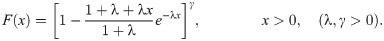
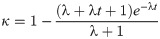
Recently, many researchers have suggested new generalization for life time distributions used in statistics and possess flexibility in applications. Although the wide range of applications of the Lindley distribution [1] has a wide range of applications, it does not provide a good fit for modeling phenomenon with non-monotone failure rates, such as bathtub upside down failure shaped. For this lack of flexibility, many authors proposed a new generalizations of the traditional Lindley distribution by adding one or more shape parameters to add more flexibility to the PDF and the hazard rate function. Extended generalized Lindley (EGL) distribution is a very important lifetime and survival distribution which can be used as an effective alternative to the well known distributions such as generalized Lindley (GL), Lindley (L) and exponential distributions. It has different applications in modelling various types of data including economics and actuarial sciences data because its hazard rate can be increasing, decreasing, upside down bathtub shaped and unimodal. In addition, this model presented a better fit to data resulting in accurate results and predictions, which should facilitate better public policy in a wide range of areas including medicine, genetics, environmental health, reliability, survival analysis and actuarial sciences data because its hazard rate can be increasing, decreasing, upside down bathtub shaped and unimodal. Several types of lifetime model distribution have been proposed in literature. Zakerzadah and Dolati [2] presented GL distribution and studied its statistical properties and applications. Also, Oluyede and Yang [3] introduced a new class of GL distributions with applications. Nadarajah et al. [4] introduced GL distribution with shape and scale parameters γ, λ, respectively, the probability density function (PDF) is given by

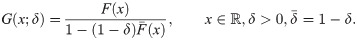
On the other hand, Marshall and Olkin [5] proposed a method of adding a new shape parameter to any well-known distribution whose cdf denoted by F(x), as follows

2 New family and its own sub-models

This section proposes the new family distribution and derives density and survival functions from this family.

2.1 New family description

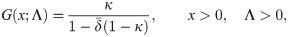
Let Λ = (λ, γ, δ) and inserting Eq (2) in Eq (3), a new distribution denoted as EGLD (x;Λ) can be obtained. Then, the CDF of the EGLD can be obtained as;

where $$ \kappa ={(1-\frac{(\lambda +\lambda x+1)e^{-\lambda x}}{\lambda +1})}^{\gamma }$$.

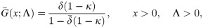
The corresponding survival function (SF) and the PDF are defined by

and

respectively. The next proposition presents the behavior of the pdf of the EGLD (x;Λ) with various choices of parameters.

Proposition 2.1. Let X ∼ EGLD (x;Λ), then:

If γ < 1, then X has a decreasing pdf.

If γ ≥ 1, then X has an increasing pdf.

If γ ≥ 1, then X upside-down bathtub shaped.

Fig (1) shows the various shapes of the PDF of the EGLD given by Eq (6) by choosing the scale parameter, λ, to be 2.90 in all the cases and different values of the shape parameters. Fig (1) indicates that the proposed distribution is suitable to model the right skewed data.

Fig 1

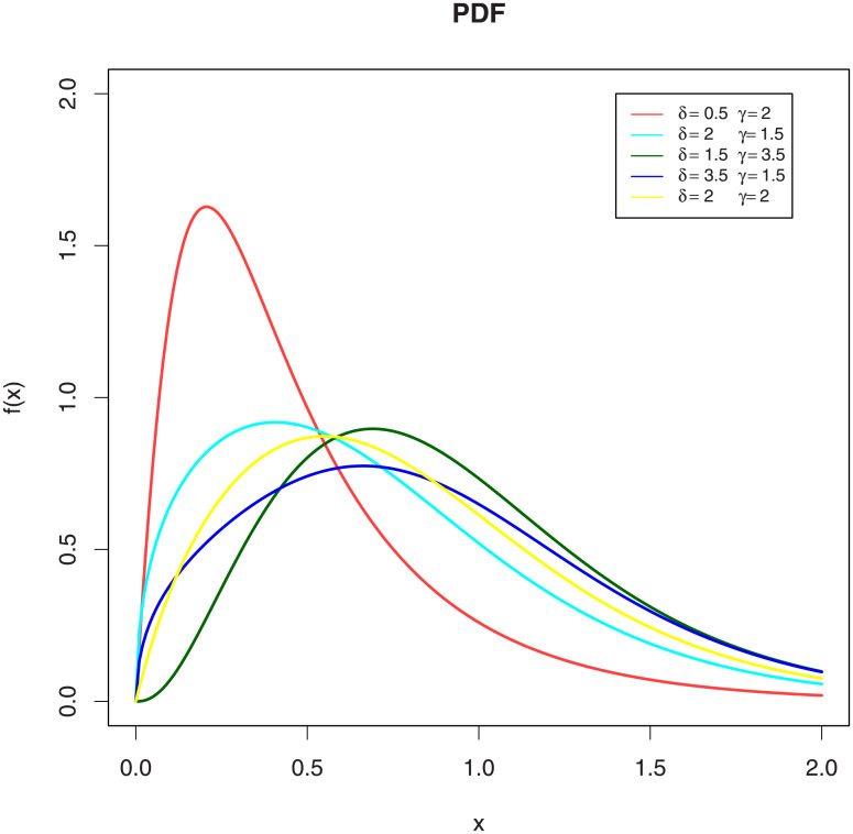
Plots PDF of the EGLD with λ = 2.9.

Figure (1) shows the various shapes of the PDF of the EGLD given by Eq (6) by choosing the shape parameter, λ, to be 2.90 in all the cases and different values of the shape parameters. Figure (1) indicates that the proposed distribution is suitable to model the right skewed data.

3 Reliability and statistical properties

In this section, reliability and some statistical properties of the EGLD are presented, especially quintile function, moments, (reversed) failure rate, mean residual life, order statistics and stochastic orderings.

3.1 Failure rate and mean residual life

Let T ≥ 0 be a continuous random variable with cdf F(t) and pdf f(t), the failure rate (FR) function of the EGLD is defined as

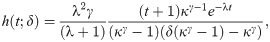
For the EGLD, the failure rate function h(t) is

where

Proposition 3.1. Let h(t) be the failure rate function of a random variable T distributed according to EGLD (Λ). Then

h(t) is increasing for λ < 1 and γ > 1.

h(t) is bathtub shaped for λ > 1 and γ > 1.

h(t) is decreasing for λ < 1 and γ < 1.

The mean residual life (MRL) can be obtained by general formula (see Navarro et al. [14])

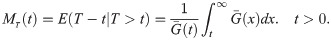
Lemma 3.2. Let T ∼ EGLD (t;Λ), then the MRL function of a lifetime random variable is given by:

where

and

be the upper incomplete gamma, for more details, see Wall [15].

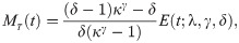
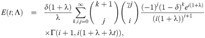
Fig (2) shows the different shapes of its FR and MRL for some selected parameters values with scale parameter one. This Figure indicates that the EGLD FR can be monotonically increasing and MRL can be monotonically decreasing.

Fig 2

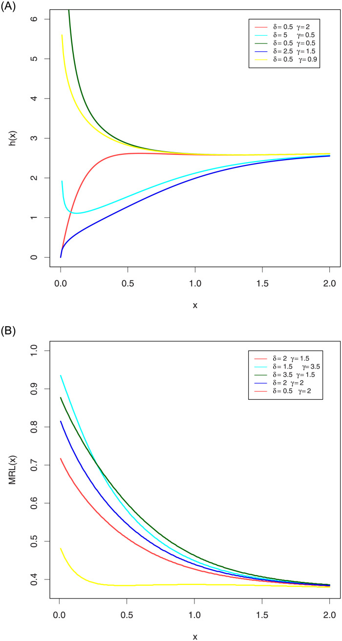
Plots FR and MRL of the EGLD with λ = 2.9.

Figure (2) shows the different shapes of its FR and MRL for some selected parameters values with scale parameter one. This Figure indicates that the EGLD FR can be monotonically increasing and MRL can be monotonically decreasing.

3.2 Reversed failure rate and mean inactivity time

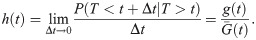
For a continuous distribution with pdf, g(t), and CDF, G(t), the failure rate function, also known as the reversed failure rate (RHR) function, is defined as

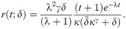
For the EGLD, the reversed failure rate function r(t) is

For a continuous distribution with pdf g(t) and cdf G(t), the mean inactivity time (MIT) function is defined as

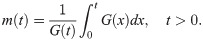
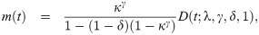
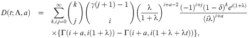
For the EGLD, the mean inactivity time function m(t) is

where

For a continuous distribution with pdf g(t) and CDF G(t), the strong mean inactivity time (SMIT) function is defined as

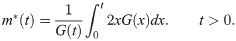
For the EGLD, the strong mean inactivity time function m* is

Fig (3) shows the different shapes of its RHR and MIT for some selected parameters values with scale parameter one. This Figure indicates that the EGLD RHR can be monotonically decreasing and MIT can be monotonically increasing.

Fig 3

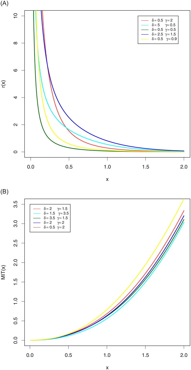
Plots RHR and MIT of the EGLD with λ = 2.9.

Figure (3) shows the different shapes of its RHR and MIT for some selected parameters values with scale parameter one. This Figure indicates that the EGLD RHR can be monotonically decreasing and MIT can be monotonically increasing.

3.3 Renyi entropy

Entropy has been used in areas like physics (sparse kernel density estimation), medicine (molecular imaging of tumors) and engineering (measure the randomness of systems). The entropy is a measure of variation of the uncertainty of a random variable X with density function f(x). The Rényi entropy (RE) [16] of order b is defined as

For the EGLD(x;Λ) in (6) can be obtained as

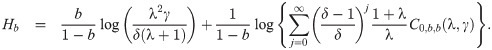
Table 1 present the critical points of the reliability functions of the EGLD. These values can be determined numerically using R and Maple¹⁴.

Table 1

Critical points of reliability functions for selected values of λ = 2.90 and γ = 3.00 at t = 0.5.

δ	030	0.50	0.65	0.80	0.95	1.00
HR	2.93562	2.31981	2.00445	1.76457	1.57597	1.52176
MRL	0.354484	0.398896	0.428236	0.454937	0.479475	0.487237
RHR	1.94233	2.55815	2.8735	3.11338	3.30198	3.3562
MIT	0.2035	0.18559	0.178116	0.173002	0.169276	0.168248
SMIT	0.149169	0.138466	0.133869	0.130681	0.128335	0.127684
Renyi entropy	0.625869	0.739825	0.794179	0.835126	0.867617	0.877068

From Table 1 we have the following observations:

For fixed λ and γ, the HR, MIT and SMIT of the different parameters decrease as δ increases.

For fixed λ and γ, the MRL and RHR of the different parameters increases as δ increases.

3.4 Quantiles and moments

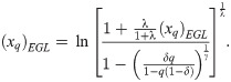
Lemma 3.3. Let X ∼ EGLD (x;Λ). Then, the qth quantile function, denoted bt (x_q)_EGL, is given by

Remark 3.4

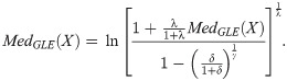
The median of the EGLD (x;Λ) as



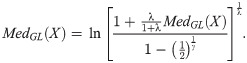
The qth quantiles of the GL (x;λ, γ) model as



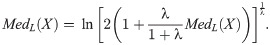
The qth quantiles of the L(x;λ) model as

The next lemma are need in the noncentral moment of the EGLD.

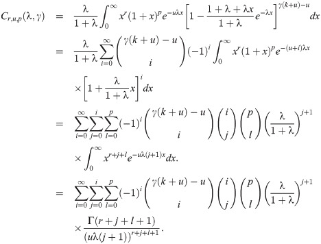
Lemma 3.5. For λ > 0 and γ > 0. Let

we have

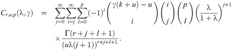
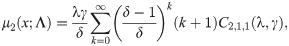
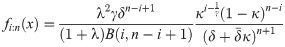
Proposition 3.6. Let X∼ EGLD (x;Λ). Then, the noncentral moment of X has the following form:

assuming that Λ > 0.

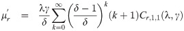
Based on proposition (3.6), the following measures hold for every Λ > 0 of the EGLD (x;Λ).

and the variance of the EGLD (x;Λ) as

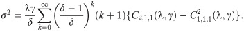
The measures of skewness and kurtosis are computed using the following expressions:

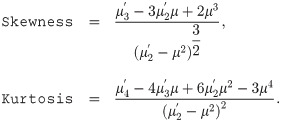
Table 2 lists the first six moments, variance, skewness and kurtosis for the EGLD (x;Λ) for some selected values for δ by choosing the scale and shape parameters to be one in all cases.

Table 2

Moments of the EGLD for some parameter values, λ = 2.90 and γ = 3.00.

$$	δ = 0.30	δ = 0.65	δ = 0.80	δ = 1.00
$$	0.518682	0.679073	0.727784	0.782748
$$	0.40514	0.65132	0.735537	0.835731
$$	0.450433	0.828127	0.968904	1.1432
$$	0.669297	1.33013	1.59089	1.92291
$$	1.2536	2.59797	3.1476	3.86051
$$	2.82781	5.98913	7.30897	9.04088
Variance	0.13611	0.190179	0.205868	0.223037
Skewness	1.97349	1.53782	1.4339	1.32789
Kurtosis	9.26325	6.76956	6.28049	5.82284

From Table 2 we have the following observations:

For fixed λ and γ, the Skewness, and Kurtosis of the different parameters decrease as δ increases.

For fixed λ and γ, the moments and Variance of the different parameters increases as δ increases.

3.5 Order statistics

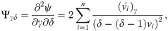
Order statistics have various applications in many different areas of statistical theories and applications such as quality control testing and reliability. Let X₁, …, X_n be a random sample of size n from the EGLD (x;Λ). The PDF of the i^th order statistic, X_{i: n}, is defined by

where B(.,.) is the beta function. Also, the joint pdf of the (i, j)^th order statistic, X_{i: n}, X_{j: n} and 1 ≤ i ≤ j ≤ n, is defined by

where $$ {\kappa }_s={(1-\frac{1+\lambda +\lambda x_s}{\lambda +1}{e}^{-\lambda x_s})}^{\gamma }$$ and $$ \epsilon =\frac{n!}{(i-1)!(j-i-1)!(n-j)!}.$$

3.6 Stochastic orderings

Stochastic orders has many applications in different fields such as income, actuarial science, wealth inequality, engineering, medical and biological sciences, lifetime, queuing theory and reliability analysis (Shaked and Shanthikumar [17]). Let X₁ and X₂ be univariate random variables with distribution functions G₁(x) and G₂(x) and reliability functions $$ {\overline{G}}_1\left(x\right)$$ and $$ {\overline{G}}_2\left(x\right)$$, respectively, with corresponding probability densities g₁(x), g₂(x).

If G₁(x)≥G₂(x), ∀x, then X₁≤_st X₂ (stochastically ordering).

If g₁(x)≥g₂(x), ∀x, then X₁≤_lr X₂ (likelihood ratio ordering).

If h₁(x)≥h₂(x), ∀x, then X₁≤_hr X₂ (hazard rate ordering).

If m₁(x)≥m₂(x), ∀x, then X₁≤_mrl X₂ (mean residual life ordering).

If G₁(x)/G₂(x) is decreasing, ∀x, then X₁≤_rhr X₂ (reversed hazard rate ordering).

From the last stochastic orders, the following implications are satisfied (Shaked and Shanthikumar [17]):

The next theorem propose the EGLD are ordered with respect to the strongest likelihood ratio ordering when suitable assumptions are satisfied.

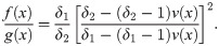
Theorem 3.7. Let X and Y be univariate random variables such that X ∼ EGLD(λ, γ, δ₁) and Y ∼ EGLD(λ, γ, δ₂) If δ₁ < δ₂, then

4 Maximum likelihood estimates

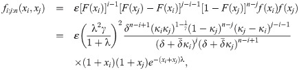
Let x = (x₁, x₂, …, x_n) of a random sample of size n from EGLD with three parameters (Λ = (λ, γ, δ)). The log-likelihood function (LLF) takes the form

The MLEs of the unknown parameters λ, γ and δ can be obtained by solving the

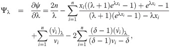
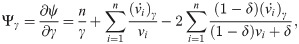
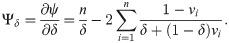
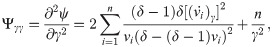
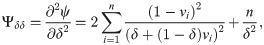
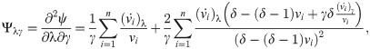
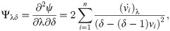
These equations can be solved numerically by using statistical software. The asymptotic confidence intervals (CIs) for the parameters of EGLD(Λ) distribution are given according to the asymptotic distribution of the maximum likelihood estimates (MLEs) of the parameters. For more details about the maximum likelihood estimates see for example Dong et al. [18], Chen et al. [19] and Chen et al. [20]. The second derivatives of the LLF of EGLD with respect to Λ are given in the Appendix part [B], from Eqs (41)–(46). The estimators are approximately bi-variate normal with mean Λ and the observed information matrix is given by

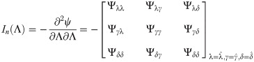
The 100(1−ϑ)% approximate two-sided confidence intervals (CIs) for the parameters λ, γ and δ are

5 Simulation study

In this section, a simulation study by considering different parameters values and different samples sizes is conducted to decide which estimation method provides the best estimates in terms of minimum mean square error (MSE). The samples sizes are selected to be 30, 50, 70, 100, 150 and the parameters values are selected to be (λ, γ, δ) = (2.90, 3.00, 0.70)and(0.20, 2.70, 0.90). The process is replicated 1000 times for each setting and the average estimates,the average Bias and the average MSEs are computed. For more details about the MSEs see for example Zeng et al. [21], Zeng et al. [22], Zeng et al. [23] and Zeng et al. [24]. These values are tabulated in Table 3. The results in these tables show that the four estimation methods provide an asymptotically unbiased estimates where the estimates tend to the true parameters values as the sample size increases. Also it is noted that the MSEs decreases in all the cases for the different estimates as the sample size increases. In addition, the simulation results shows that the LSEs have the smallest MSEs in most of the cases.

Table 3

Simulated average estimates (AEs) (first row), mean squared errors (MSEs) (second row) and bias estimates (third row) under different settings parameters.

EGLD(λ, γ, δ)	n	Estimates	λ	γ	δ
EGLD(2.90,3.00,0.70)	30	Est.	3.32791	2.96355	1.21411
		MSE	2.74349	1.89877	2.61318
		Bais	0.42791	-0.03645	0.51411
	50	Est.	3.19317	2.82378	1.13280
		MSE	0.92870	1.12008	1.93396
		Bais	0.29317	-0.17622	0.43280
	70	Est.	3.06135	2.92424	0.96370
		MSE	0.65713	0.84221	1.01533
		Bais	0.16135	-0.07576	0.26370
	100	Est.	3.04659	2.86435	0.93394
		MSE	0.48586	0.58779	0.73386
		Bais	0.14660	0.13565	0.23394
	150	Est.	2.99243	2.95314	0.84701
		MSE	0.30126	0.36852	0.32648
		Bais	0.09243	0.04687	0.14709
EGLD (0.20,2.70,0.90)	50	Est.	0.21920	2.63306	1.71376
		MSE	0.00315	0.75398	3.20126
		Bais	0.01920	-0.06694	0.81376
	100	Est.	0.21147	2.61271	1.40693
		MSE	0.00191	0.37813	1.45407
		Bais	0.01147	-0.08729	0.50693
	150	Est.	0.20638	2.68321	1.21072
		MSE	0.00101	0.24497	0.79587
		Bais	0.0064	-0.01679	0.31072

6 Application: Waiting time

The next data set studied the service of 100 bank customers and waiting times (in minutes). These data were considered by Ghitany et al. [25] and given by Table 4.

Table 4

The data set of waiting time presented.

0.8	0.8	1.3	1.5	1.8	1.9	1.9	2.1	2.6	2.7	2.9	3.1	3.2	3.3	3.5
3.6	4.0	4.1	4.2	4.2	4.3	4.3	4.4	4.4	4.6	4.7	4.7	4.8	4.9	4.9
5.0	5.3	5.5	5.7	5.7	6.1	6.2	6.2	6.2	6.3	6.7	6.9	7.1	7.1	7.1
7.1	7.4	7.6	7.7	8.0	8.2	8.6	8.6	8.6	8.8	8.8	8.9	8.9	9.5	9.6
9.7	9.8	10.7	10.9	11.0	11.0	11.1	11.2	11.2	11.5	11.9	12.4	12.5	12.9	13.0
13.1	13.3	13.6	13.7	13.9	14.1	15.4	15.4	17.3	17.3	18.1	18.2	18.4	18.9	19.0
19.9	20.6	21.3	21.4	21.9	23.0	27.0	31.6	33.1	38.5.

To show the applicability of the proposed distribution and the different estimators presented in the previous sections one real data set is analyzed and shows the significance of our new distribution. We compare the results of the EGLD with GL and L distributions. We first use the maximum likelihood method to estimate the unknown parameters of the competitive distributions. These estimates are displayed in Table 5.

Table 5

The estimates of parameters corresponds to data set.

Distribution	parameter MLEs
	$$	$$	$$
EGLD	0.172494	1.46019	0.461444
GLD	0.210779	1.27729	-
LD	0.186571	-	-

The observed information of the data and the asymptotic covariance matrix of MLEs, respectively, are

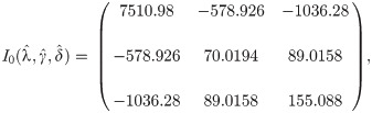
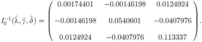
Therefor, 95% two-sided asymptotic confidence intervals for the parameters λ, γ, and δ respectively, are [0.161736,0.183251], [1.40029, 1.52008] and [0.374721, 0.548166]. Some goodness of fit measures are displayed in Table 6. From this table we can note the following:

According to maximum log-likelihood criterion for goodness of fit and −logL, the order of best fit for the above models is: Best EGLD ⇒ GLD ⇒ LD Worst.

To compare the different models with the EGLD we obtain the Kolmogorov-Smirnov (K-S) statistic as well as its p-value. These statistics are displayed also in Table 7 for the data set. From these results, we can conclude that the EGLD has the K-S value 0.040985 and the highest p-value 0.956357 among all other competitive models, therefore it can be selected as the best model.

According to A and W, the order of best fit for the above models is: Best GLD ⇒ LD ⇒ EGLD Worst.

According to these statistics, the EGLD model fits the current data set better than the other models.

Table 6

Goodness-of-fit statistics corresponds to data set.

Distribution	−logL	K−S	A	W
		(p-value)	(p-value)	(p-value)
EGLD	317.155	0.040985	0.129516	0.0185372
		(0.956357)	(0.991705)	(0.982528)
GLD	317.803	0.0471189	0.240452	0.037585
		(0.855563)	(0.784184)	(0.721155)
LD	319.037	0.0495455	0.267223	0.0419412
		(0.799012)	(0.706235)	(0.645525)

Table 7

Likelihood ratio test and its p-value corresponds to data set.

Distribution	Null hypothesis (H0)	Alternative hypothesis (H1)	LRT	(p-value)
GL	H0: δ = 1(GL)	H1: δ ≠ 1(EGLD)	19.5512	9.79415×10−6 < 0.05)
L	H0: δ = 1, γ = 1(L)	H1: δ ≠ 1, γ ≠ 1(EGLD)	4.9492	0.0261028 < 0.05)

In order to see how well the EGLD fits this data, we introduce the hypotheses test statistic as well as its p-value. The hypotheses are as follows:

Furthermore, likelihood ratio test (LRT) has been used to determine the appropriateness of the model. The hypotheses are as follows:

According to these statistics, the calculated LRT statistic is greater than the critical point for this test, which is 9.210; also, the p-value is small. furthermore, we conclude that this data fits the EGLD much better the GL and L distributions. Fig (4) shows plots of the estimated cumulative and estimated densities of the fitted models for the data data described below.

Fig 4

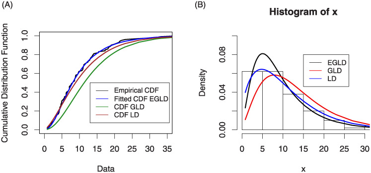
Plots estimated CDF and PDF of models for the data set.

Figure (4) shows plots of the estimated cumulative and estimated densities of the fitted models for the data data described below.

Concluding remarks

Introducing a new model of the EGLD is the main goal of this article. This model has the characteristic of being capable of failure criteria and modeling various shapes of aging. The proposed distribution contains one scale and two shape parameters. The distributions GL, L and among others are sub-models of the EGLD and studied in this article. Some statistical properties of the new distribution are discussed. estimation methods are used to estimate the unknown parameters of the proposed distribution. The efficiency of the different estimators are compared via simulation study in terms of minimum mean square errors. The simulation study shows that the least square estimates perform better than other proposed methods. Finally, two real data sets are analyzed showing that the new distribution is very competitive as compared to some well known distribution with three or more than three parameters. A future work is to estimate procedures of stress-strength reliability for Generalized Lindley Distribution. Another future work is to study and compare the Bayesian estimation based on maximum likelihood and based on maximum product of spacing to estimate the stress-strength reliability of Generalized Lindley Distribution.

Appendix

[A] Proofs of lemma and theorem.

Proof of Lemma 3.5

By changing $$ {\sum }_{i=0}^{\infty }{\sum }_{j=0}^i$$ to $$ {\sum }_{j=0}^{\infty }{\sum }_{i=j}^{\infty }$$, in the last equation and hence, the proof is completed.

Proof of Theorem (3.7)

First note that

Since, δ₁ < δ₂,

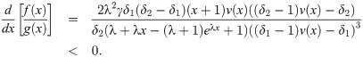
Hence, f(x)/g(x) is decreasing in x. That is X≤_lr Y. The remaining statements follows from the implications Eq (31).

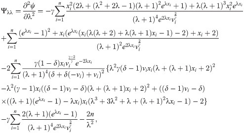
[B] The entries of the FIM for EGL distribution with respect to λ, γ and δ are given by the following equations: