1 Introduction

The importance of the nonlinear phenomena of differential equations (DEs) in sciences (biology, physics and chemistry) is significant. In any branch of natural sciences, there exists a small number of problems, that can be solved in a direct way. So, to understand the complete physical phenomena, the mathematical modeling comes into account by means of partial differential equations (PDEs), that shows an exceptional performance in science and engineering. The concept of the physical phenomena, depends upon the nature of the solutions of PDEs, so to find the solutions of PDEs, the analytical, semi analytical and numerical methods are introduced. It has been a requirement to choose a competent mechanism that adopts such mathematical models which cover physical processes as well [1].

In nonlinear sciences and engineering, analytical solutions to nonlinear PDEs have a great significance but sometimes, it becomes much problematic to deal with, that becomes a hurdle in finding analytical solutions to these DEs. So, the scientists have introduced many techniques like perturbation methods, approximation methods and numerical methods to overcome the problems of such DEs. Considering the effect of nonlinearity, many analytical techniques concentrate on linearizing the physical phenomena, that yields the variation in the nature of these analytical solutions from the actual ones and becomes a cause of change in the real physics of the given phenomena [1].

Several efforts have been exerted for finding and improving the dynamic, robust and effective schemes to solve the nonlinear PDEs (KdV equation, Burgers’ equation, KdV Burgers’ equation, Helmholtz equation, Schrödinger equation, Klein-Gordon equation, diffusion equation, sine-Gordon equation and Fisher’s equation), for example inverse scattering scheme, homotopy perturbation method, tanh-sech method, F-expansion method, sine-cosine method, tanh-function method, Hirota’s bilinear method, exp-function method, Jacobi elliptic functions method, (G/G’)-expansion method, Riemann-Hilbert approach and many more [2, 3–10].

Kortweg-de Vries (KdV) equation is a nonlinear PDE, that is used to model travelling waves in shallow water and harmonic crystal. KdV was proposed by Boussinesq about 1877 and determined by Kortweg-de Vries about 1895. Moreover, the well known KdV equation of order seven was introduced by Pomeau et al. [11] in a research paper, to study its stability underneath a singular (restricted) perturbation. These days, the development of KdV equation is important in the phenomena of fluid dynamics, magma flow, conduit waves, optical fibers, waves in plasma physics and flow in blood vessels. The significance of KdV does not exist in their utilization only but also in some sort of belongings that are not normally anticipated by nonlinear PDEs. Moreover, KdV can have multi-soliton solutions along solitary wave solutions, when these interesting facts about KdV had been introduced, many authors presented the initial value problem associated to the KdV from theoretical and numerical point of view [12, 13].

In literature, there exist many analytical and numerical schemes like He’s variation iteration method, pseudospectral method, Adomian decomposition method (ADM), Bäcklund transformations to solve such problems, finite difference method (FDM), finite element method (FEM), finite volume method (FVM), homotopy analysis method (HAM), Fourier spectral method (FSM) and variation iteration method (VIM) to solve such problems [1, 2, 14–17], some of them are given by:

Arora and Sharma [1] approximated the seventh order KdV equations for example Sawada-Kotera-Ito equation, Lax equation and Kaup-Kuperschmidt equation by HAM. They used a parameter namely h to control the convergence of the method and by fixing it, the computational results were compared with the analytical solutions. That indicated the robustness and elegance behavior of the proposed scheme.

Darvishi et al. [2] solved the Lax’s seventh-order KdV equation by pseudospectral method. Darvishi’s preconditioning was used for the accuracy of matrix vector multiplication. There was a good agreement observed between numerical solution and exact solution. Saravi et al. [14] reconstructed the variational iteration method (VIM) for the numerical solution of Lax’s and Sawada-Kotera equations of order seven. They compared the results with the Adomian decomposition method (ADM) and existing analytical solutions. The computational outcomes indicated the effectiveness of VIM for both equations.

Aljahdaly [18] presented two applications of Lax-equation and Kaup-Kuperschmidt equation of order seven by constructing new travelling wave solutions. Moreover, nonlinear PDEs were solved analytically by modified auxiliary equation, that resulted the stable analytical solutions. Ganji and Abdollahzadeh [19] solved a nonlinear evolution equation analytically. The sech-method and the exp-function method were used to form the solitary travelling wave solutions of Lax’s (KdV) equation of order seven, that were important from physical point of view.

Sharma and Arora [20] established the modified form of He’s variational iteration method (MVIM) to solve some non-linear partial differential equations analytically, such as Fisher-type equation, cubic Boussinesq equation and Caudrey-Dodd-Gibbon equation of order seven. The numerical results indicated the efficient behavior of the prescribed method. The strength of MVIM over standard form of VIM was investigated, as it assured less computational cost. Salas implemented Cole-Hopf transform for construction of analytical solutions for generalization of Lax’s KdV equation and the Sawada-Kotera-Ito KdV equation of order seven with forcing term [21].

Since the frequently used techniques involve FDM, FEM, FVM and FSM for the approximation of DEs. Along with many benefits these numerical methods were facing some deficiencies, that encouraged the mathematicians to do struggle for more better numerical schemes and a wide range of numerical schemes including wavelet schemes were introduced. The wavelet techniques are widely used to avoid the complications of science and engineering [22, 23] and advantageous over FDM, FEM, FVM and FSM.

The word wavelet was coined by Morlet and Grossmann [24] and the analysis about wavelets was presented by Morlet, Grossmann and Meyer and gained a great success in the field of wavelets [24, 25]. Mallat gave the idea of multiresolution analysis (MRA), that used to provide high resolution for simulation of nonlinear and singular equations [26]. In 1988, Daubechies introduced a scheme with wavelets having compact support and scaling functions [26]. The appealing features of wavelet methods include coping with the singularities, rough structures and unstable phenomena, that are exhibited by the analyzed equations. In addition, for the numerical solution of PDEs wavelets are established on collocation procedure and Galerkin techniques.

For approximation of PDEs, the authors have used many wavelet techniques but Haar wavelet (HW) is considered simple and efficient among them. Many models in different eras of science and engineering are constructed with the aid of HW [27]. Alfred Haar was the founder of HW, he introduced it in 1909 [28].

Haar functions are built up on piecewise constant functions with orthonormal basis. Due to their behavior of compact support, they become zero after a finite interval. So, being local they can easily handle irregularities, that’s why HW is considered preferable over other wavelets. In addition, HW is a special case of wavelet introduced by Daubechies [29].

The derivatives of HW functions fail to exist at the points of discontinuities, that become the reason of failure of applying HW directly to solve PDEs, to sort out this difficulty, the integration of wavelets has been introduced [27]. The techniques of HW functions have been tested in different fields like to denoise the noisy data, for analyzing the time frequency and for approximation of linear and nonlinear differential, integro-differential and integral equations [30–42].

Aziz et al. introduced quadrature rules for the of double and triple integrals on the basis of HW and compound functions. The presented technique was observed more accurate and flexible in comparison with the techniques existing in the literature by finding absolute errors [43].

Lepik solved nonlinear evolution equations numerically by a scheme based on HW functions. The author applied HW method on Burgers’ and sine-Gordon equations and compared the obtained and already existing results in the literature. It was noticed, that the proposed method was computationally economical [44]. The general form of seventh-order KdV-type equations is given by [18, 45]:

This form is the universal model for the study of shallow water waves along-with surface tension and magneto-acoustic waves in plasma. In the current study, we will explore the special types of this equation which are given below:

For α = 140, β = 70, γ = 280, μ = 70, ν = 70, ϕ = 42 and ψ = 14, it is called Lax equation of order seven:

For α = 252, β = 63, γ = 378, μ = 126, ν = 63, ϕ = 42 and ψ = 21, it is called seventh-order Sawada-Kotera (SK) equation:

For α = 2016, β = 630, γ = 2268, μ = 504, ν = 252, ϕ = 147 and ψ = 42, it is called Kaup-Kuperschmidt (KK) equation of order seven:

The seventh order KdV-type equations are utilized to study different nonlinear phenomena of physical situations and its role is significant in the phenomena of wave propagations [46].

The aim of this research work is to choose an authentic approximation of seventh-order KdV-type equations (Lax, Sawada-Kotera-Ito and Kaup-Kuperschmidt equations) using one-dimensional Haar wavelet collocation method (1-D HWCM), that provides high quality computed results in short time with a few grid points.

The proposed research work is a part of thesis [47] and it is arranged in the subsequential style. In Section 2, the definitions of MRA and HW are given. In Section 3, the proposed numerical method for seventh-order KdV-type equations is demonstrated. In Section 4, the convergence theorem of the HW is discussed. The computed results are reported in Section 5. Finally, in Section 6, a few concluding remarks of the research work are presented.

2 Materials and methods

2.1 Multi-resolution analysis

The concept of wavelets becomes clear via multi-resolution analysis (MRA), where f is considered a function from the class of all square integrable functions over the real line, doing MRA of L₂(R), $$ {\tilde{\chi }}_{\tilde{m}},{\tilde{\chi }}_{\tilde{m}+1},\dots $$ of subspaces can be generated in a way that the projection of f onto these spaces gives finer approximations of the function f as $$ \tilde{m}\to \infty .$$ MRA of L₂(R) yields $$ {\tilde{\chi }}_{\tilde{m}}\subset L_2\left(R\right)$$, $$ \tilde{m}\in Z$$ that is a sequence of closed subspaces, with the following properties:

Monotonicity $$ \cdots \subset {\tilde{\chi }}_{-1}\subset {\tilde{\chi }}_0\subset {\tilde{\chi }}_1\subset \dots $$

$$ {\tilde{\chi }}_{\tilde{m}}\text{s}$$ fulfill the condition that $$ {\bigcup }_{\tilde{m}\in Z}{\tilde{\chi }}_{\tilde{m}}$$ is dense in L₂(R) and $$ {\bigcap }_{\tilde{m}\in Z}{\tilde{\chi }}_{\tilde{m}}=0$$.

If $$ f\left(x\right)\in {\tilde{\chi }}_0$$, then $$ f\left(2^{\tilde{m}}x\right)\in {\tilde{\chi }}_{\tilde{m}}$$. In other words, this statement indicates that $$ {\tilde{\chi }}_{\tilde{m}}s$$ can be obtained from the central space $$ {\tilde{\chi }}_0$$ by the process of scaling.

If $$ f\left(x\right)\in {\tilde{\chi }}_0$$, then $$ f(2^{\tilde{m}}x-\tilde{n})\in {\tilde{\chi }}_{\tilde{m}}$$. In other words, $$ {\tilde{\chi }}_{\tilde{m}}s$$ remain unchanged when the process of translation is applied to them.

A function $$ \tilde{\varphi }\in {\tilde{\chi }}_0$$ is obtained in a way that the set $$ \{\tilde{\varphi }(x-\tilde{n}):\tilde{n}\in Z\}$$ forms a Riesz basis in $$ {\tilde{\chi }}_0$$.

The approximation of general functions is performed with the help of the space $$ {\tilde{\chi }}_{\tilde{m}}$$ by defining proper projection (of these functions). Any square integrable function in L₂(R) may be approximated arbitrarily closed by using these projections due to the property, that is the union of $$ {\tilde{\chi }}_{\tilde{m}}\text{s}$$ is closed in L₂(R). For instance, if the space $$ {\tilde{\chi }}_{\tilde{m}}$$ is defined as:

then after translation and dilation, MRA may be formed for the sequence of spaces $$ \{{\tilde{\chi }}_{\tilde{m}},\tilde{m}\in Z\}$$ given by Eqs (8) and (10) by using the scaling function ς₁(x). It is noticeable, that for all $$ \tilde{m}$$, the space $$ {\tilde{\varrho }}_{\tilde{m}}$$ is an orthogonal complement of $$ {\tilde{\chi }}_{\tilde{m}}$$ in $$ {\tilde{\chi }}_{\tilde{m}}+1$$, which means that w.r.t. any given inner product, the space $$ {\tilde{\varrho }}_{\tilde{m}}$$ contains all those functions in $$ {\tilde{\chi }}_{\tilde{m}}+1$$ which are orthogonal to all those in $$ {\tilde{\chi }}_{\tilde{m}}$$. The basis which is formed by the set of functions for the space $$ {\tilde{\varrho }}_{\tilde{m}}$$ is called a formation of wavelets [26].

2.2 Haar wavelet

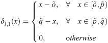
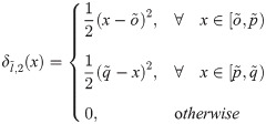
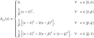
The HW functions are the functions with compact support, they are based on bounded intervals and are defined on [0, 1). These functions (except Haar scaling function) are with unique representation given as [27]:

with

where $$ \tilde{l}$$ is used for wavelet number, $$ \tilde{o},\tilde{p}$$ and $$ \tilde{q}$$ are constants, $$ \tilde{n}$$ is the translation parameter and $$ \tilde{r}$$ is used for determining the resolution level.

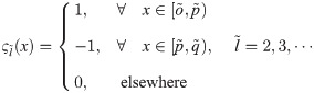
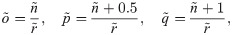
For approximation by HW functions, MRA performs a great role, here, $$ \tilde{M}$$ is used for maximum level of resolution, whereas, the level of HW is taken as the integral values of $$ \tilde{m}$$ with $$ \tilde{m}=lo{g}_2\tilde{r}$$, that implies $$ \tilde{r}=2^{\tilde{m}}$$ with $$ \tilde{m}=0,1,2,...,\tilde{M}$$. Moreover, the wavelet number $$ \tilde{l}$$ satisfies the relation $$ \tilde{l}=\tilde{r}+\tilde{n}+1$$, by taking $$ \tilde{l}=2$$, we are with ς₂(x), that is mother wavelet (HW function). The father wavelet (Haar scaling function) ς₁(x), has the following representation:

Any member of the family of square integrable functions defined on [0, 1) can be represented as an infinite sum of HW functions as:

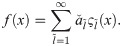
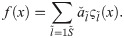
We identify the integer $$ \tilde{R}=2^{\tilde{M}}$$ and $$ \tilde{S}=2\tilde{R}=2^{\tilde{M}+1}$$, to define discrete HW functions, where $$ \tilde{M}$$ is maximum resolution level. So, any function f(x) on [0, 1) can be estimated as a finite sum of HW functions in the following manner:

The concept of Haar integrals were derived by Chen and Hsiao in 1997 [48], here, the Haar integrals are presented by:

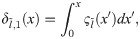
We can calculate these integrals using Eq (8) and the first two integrals are given below:

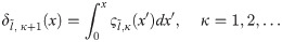
The general expression for the Haar integrals is given by

The above expression $$ {\delta }_{\tilde{l},\tilde{s}}\left(x\right)$$ is for $$ \tilde{l}=2,3,\dots $$ and $$ \tilde{s}=1,2,\dots $$, for $$ \tilde{l}=1$$ and $$ \tilde{s}=1,2,\dots $$, we have $$ {\delta }_{\tilde{l},\tilde{s}}\left(x\right)=\frac{x^{\tilde{s}}}{\tilde{s}!}$$.

3 The proposed approximation method

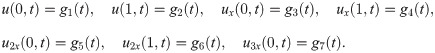
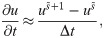
The presented technique is constructed on the basis of FDM and 1-D HWCM for Eq (1). The space derivatives in Eq (1) are discretized using 1-D HWCM, whereas, the discretization of the temporal derivative in Eq (1) is enforced using FDM, that is:

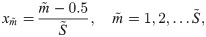
Now, applying finite difference scheme to the KdV Eq (1)

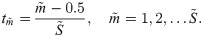
Linearizing the nonlinear terms of Eq (17), we have

After simplifications, we have

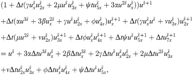
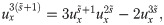
Now applying CPs, we have

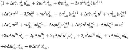
The highest order partial derivative occurring in Eq (1) can be approximated using HW functions as:

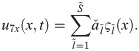
Integration of Eq (21) w.r.t. x yields the interpretations for the other derivatives and the function i.e. u(x, t) as:

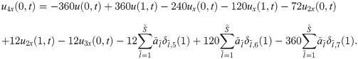
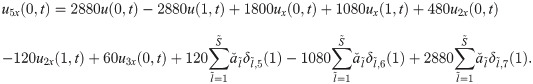
The expressions for the unknowns u_4x(0, t), u_5x(0, t) and u_6x(0, t) are calculated by integrating Eqs (25), (26) and (27) w.r.t. x from 0 to 1 as:

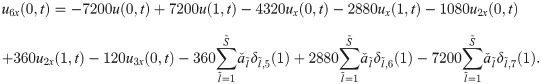
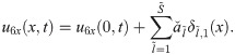
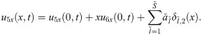
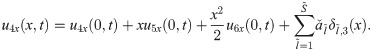
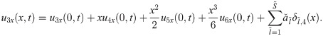
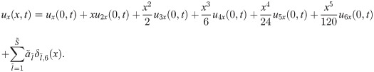
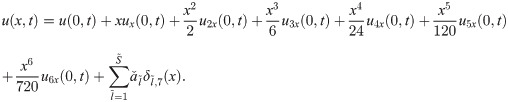
Substituting all the above expressions in Eq (20), we obtain a system of equations. In this system of equations, the known values of u_k’s at time $$ t_{\tilde{s}}$$ are substituted to calculate the Haar coefficients for the solution at the next time $$ t_{\tilde{s}+1}$$. Actual solution at the next time is obtained using these Haar coefficients. Using this iterative process, the solution at any specific time can be obtained.

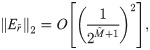
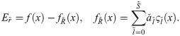
4 Convergence theorem

Theorem 1 Suppose that $$ f\left(x\right)=\frac{d^{\tilde{s}}u\left(x\right)}{d{x}^{\tilde{s}}}\in L^2\left(\mathbb{R}\right)$$ is a continuous function on [0, 1] and its first derivative is bounded:

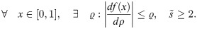
Then the HW method, based on approach proposed in [30, 49] will be convergent, i.e., $$ |E_{\tilde{r}}|$$ vanishes as $$ \tilde{M}$$ tends to infinity, the convergence is of order two:

Proof: For proof, see [30, 50].

5 Results and discussion

To analyze the validity of the presented numerical technique, some test problems are considered in this section. The maximum absolute errors (MAEs) are denoted by the symbol $$ E_c\left(\tilde{S}\right)$$. Here, all the problems are defined on the interval [0, 1].

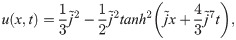
Test Problem 1 Consider the Lax equation of order seven which is given in Eq (4) with exact solution [1, 2, 45]:

Table 1

Point wise errors at Δt = 0.01 and $$ \tilde{j}=0.3$$ and $$ \tilde{S}=32$$ for Test Problem 1.

x/t	2	4	6	8	10
	Point wise error	Point wise error	Point wise error	Point wise error	Point wise error
0	0	0	0	0	0
0.1	2.0853 × 10−07	8.9657 × 10−07	2.0534 × 10−06	3.6617 × 10−06	5.6972 × 10−06
0.2	4.2940 × 10−07	2.5373 × 10−06	6.2873 × 10−06	1.1624 × 10−05	1.8469 × 10−05
0.3	6.7499 × 10−08	2.9241 × 10−06	8.9113 × 10−06	1.7807 × 10−05	2.9482 × 10−05
0.4	1.6779 × 10−06	7.0797 × 10−07	7.0813 × 10−06	1.7351 × 10−05	3.1368 × 10−05
0.5	4.1240 × 10−06	3.9311 × 10−06	5.1438 × 10−07	9.1502 × 10−06	2.1853 × 10−05
0.6	6.4536 × 10−06	9.1709 × 10−06	8.1807 × 10−06	3.4949 × 10−06	4.8213 × 10−06
0.7	7.3758 × 10−06	1.2199 × 10−05	1.4456 × 10−05	1.4111 × 10−05	1.1167 × 10−05
0.8	5.9278 × 10−06	1.0626 × 10−05	1.4055 × 10−05	1.6165 × 10−05	1.6924 × 10−05
0.9	2.4696 × 10−06	4.6532 × 10−06	6.5259 × 10−06	8.0602 × 10−06	9.2334 × 10−06
1	3.8775 × 10−14	7.5662 × 10−14	1.0966 × 10−13	1.4139 × 10−13	1.6878 × 10−13

Table 2

Maximum absolute errors at t = 1 and $$ \tilde{j}=0.3$$ for Test Problem 1.

$$	Δt = 0.1	Δt = 0.01	Δt = 0.001
	L∞	L∞	L∞
2	3.7267 × 10−06	3.7267 × 10−06	3.7266 × 10−06
4	3.8872 × 10−06	3.8874 × 10−06	3.8874 × 10−06
8	4.0451 × 10−06	4.0452 × 10−06	4.0452 × 10−06
16	4.0210 × 10−06	4.0211 × 10−06	4.0211 × 10−06
32	4.0476 × 10−06	4.0477 × 10−06	4.0477 × 10−06
64	4.0502 × 10−06	4.0503 × 10−06	4.0503 × 10−06
128	4.0498 × 10−06	4.0499 × 10−06	4.0499 × 10−06

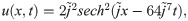
The Table 1 indicates the point wise absolute errors for different time levels. It is observed that at x = 0 and x = 1 the absolute errors are zero, whereas, the other errors are increased with the increase in time levels (by passage of time),that assures the property of time marching scheme. In Table 2, for different values of Δt (time step) and the time level t = 1, the MAEs at CPs have been calculated. The accuracy of the proposed method is measured by using different CPs, that guarantees the computational cost of 1-D HWCM is small. The point wise absolute errors are diminished up to the order 10⁻¹³ with Δt = 0.01 and x = 0.3. The MAEs are diminished up to the order 10⁻⁰⁶ and increased with the increasing time, that confirms the adequateness of the time marching scheme. It is noticeable, that after reducing the time step the accuracy of the presented scheme is increased. Moreover, the exact solution and approximate solution are shown graphically in Fig 1.

Fig 1

Comparison of approximate solution (for $$ \tilde{S}=16$$, t = 1, Δt = 0.01 and $$ \tilde{j}=0.17$$) and exact solution for Test Problem 1.

Test Problem 2 Consider the Sawada-Kotera-Ito equation of order seven given in Eq (5) with exact solution [51]:

Table 3

Point wise errors at Δt = 0.01, $$ \tilde{j}=0.4$$ and $$ \tilde{S}=32$$ for Test Problem 2.

x/t	1	5	10
	Point wise error	Point wise error	Point wise error
0	0	0	0
0.1	5.4655 × 10−09	1.0357 × 10−08	4.3205 × 10−09
0.2	5.1077 × 10−08	1.1329 × 10−07	4.9431 × 10−08
0.3	1.3776 × 10−07	3.7377 × 10−07	1.7068 × 10−07
0.4	2.0330 × 10−06	7.2330 × 10−07	3.4586 × 10−07
0.5	1.8730 × 10−06	9.9333 × 10−07	4.9760 × 10−07
0.6	9.3628 × 10−07	1.0250 × 10−06	5.8108 × 10−07
0.7	7.9367 × 10−09	7.7874 × 10−07	4.2852 × 10−07
0.8	4.4239 × 10−08	3.8274 × 10−07	2.2078 × 10−07
0.9	1.6723 × 10−08	7.4554 × 10−08	4.5079 × 10−08
1	7.7716 × 10−16	1.3878 × 10−16	3.0531 × 10−16

Table 4

Maximum absolute errors at t = 1 and $$ \tilde{j}=0.4$$ for Test Problem 2.

$$	Δt = 0.1	Δt = 0.01	Δt = 0.001
	L∞	L∞	L∞
2	1.0848 × 10−06	7.0137 × 10−07	6.5995 × 10−07
4	1.9637 × 10−06	5.3915 × 10−06	3.7997 × 10−07
8	2.1400 × 10−06	3.2034 × 10−07	1.6643 × 10−07
16	2.1656 × 10−06	2.2942 × 10−07	1.7598 × 10−07
32	2.1873 × 10−06	2.0788 × 10−07	2.0465 × 10−07
64	2.1901 × 10−06	2.0245 × 10−07	2.1203 × 10−07
128	2.1910 × 10−06	2.0088 × 10−07	2.1403 × 10−07

In Table 3, the point wise absolute errors have been calculated at the values of x = 0 to 1 and t = 1, 5, 10 for x = 0 and x = 1, it is observed that its too near to the exact solution as the absolute errors (AEs) at these two points are zero and for the other points in the interval [0, 1], the AEs are increased gradually. Moreover, in Table 4, MAEs are calculated using different CPs taking different values of time step i.e. Δt = 0.1, 0.01 and 0.001, $$ \tilde{n}=0.4$$ and t = 1.

The MAEs are decreased upto 10⁻⁰⁶ for different CPs with different time steps Δt = 0.1, 0.01 and 0.001. Moreover, the adequate behavior of the prescribed scheme may be monitored by less computational cost. It can also be noticed from the Tables 3 and 4, that the point wise errors are increased by increasing values of x and MAEs are reduced by reducing Δt.

The Fig 2, illustrates the graphical behavior of approximate solution (for $$ \tilde{S}=32$$) and exact solution.

Fig 2

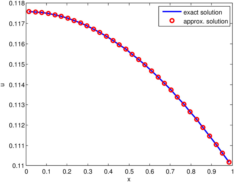
Comparison of approximate solution (for $$ \tilde{S}=32$$, t = 1, Δt = 0.01 and $$ \tilde{j}=0.21$$) and exact solution for Test Problem 2.

Test Problem 3 Consider the Kaup-Kuperschmidt equation of order seven given in Eq (6) with exact solution [1]:

The Table 5 shows the computed results of this problem. The MAEs are illustrated in Table 5, for different values of time step Δt = 0.1, 0.01 and 0.001. The MAEs are diminished upto the order 10⁻⁰⁶. Moreover, the Table 5 indicates that the property of time marching scheme is satisfied in this test problem also. The approximate solution and exact solution are presented graphically in Fig 3, that shows the vigorous behavior of the proposed scheme.

Table 5

Maximum absolute errors at t = 1 and $$ \tilde{j}=0.3$$ for Test Problem 3.

$$	Δt = 0.1	Δt = 0.01	Δt = 0.001
	L∞	L∞	L∞
2	1.4494 × 10−06	1.1149 × 10−06	1.0818 × 10−06
4	2.9750 × 10−06	1.9555 × 10−06	1.8531 × 10−06
8	3.2199 × 10−06	2.0742 × 10−06	1.9591 × 10−06
16	3.2428 × 10−06	2.0736 × 10−06	1.9562 × 10−06
32	3.2689 × 10−06	2.0893 × 10−06	1.9708 × 10−06
64	3.2710 × 10−06	2.0909 × 10−06	1.9723 × 10−06
128	3.2723 × 10−06	2.0911 × 10−06	1.9724 × 10−06

Fig 3

Comparison of approximate solution (for $$ \tilde{S}=32$$, t = 1, Δt = 0.01 and $$ \tilde{j}=0.21$$) and exact solution for Test Problem 3.

6 Conclusion

Some nonlinear PDEs of order seven are approximated including one-dimensional Lax, Sawada-Kotera-Ito and Kaup-Kuperschmidt equations. The exact solution is approximated by the one-dimensional HWCM. The proposed general equation is discretized using FDM and the collocation procedure. The proposed scheme is applied upon different test problems and an economical conduct of the scheme is investigated from the computed results. In the test problems, by reducing the time step, the accuracy is increased.