 Information theory inspired optimization algorithm for efficient service orchestration in distributed systems
PLoS ONE


Competing Interests: The authors have declared that no competing interests exist.

- Altmetric
- Introduction
- Materials and methods
- Literature review
- Proposed method
- Proposed algorithm and results
- Computational results
- Fair run and descriptive statistics
- Results from QA simulation: Initial random tour cost variable
- Results from SA simulation: Initial random tour cost variable
- Conclusion
- Supporting information
Distributed Systems architectures are becoming the standard computational model for processing and transportation of information, especially for Cloud Computing environments. The increase in demand for application processing and data management from enterprise and end-user workloads continues to move from a single-node client-server architecture to a distributed multitier design where data processing and transmission are segregated. Software development must considerer the orchestration required to provision its core components in order to deploy the services efficiently in many independent, loosely coupled—physically and virtually interconnected—data centers spread geographically, across the globe. This network routing challenge can be modeled as a variation of the Travelling Salesman Problem (TSP). This paper proposes a new optimization algorithm for optimum route selection using Algorithmic Information Theory. The Kelly criterion for a Shannon-Bernoulli process is used to generate a reliable quantitative algorithm to find a near optimal solution tour. The algorithm is then verified by comparing the results with benchmark heuristic solutions in 3 test cases. A statistical analysis is designed to measure the significance of the results between the algorithms and the entropy function can be derived from the distribution. The tested results shown an improvement in the solution quality by producing routes with smaller length and time requirements. The quality of the results proves the flexibility of the proposed algorithm for problems with different complexities without relying in nature-inspired models such as Genetic Algorithms, Ant Colony, Cross Entropy, Neural Networks, 2opt and Simulated Annealing. The proposed algorithm can be used by applications to deploy services across large cluster of nodes by making better decision in the route design. The findings in this paper unifies critical areas in Computer Science, Mathematics and Statistics that many researchers have not explored and provided a new interpretation that advances the understanding of the role of entropy in decision problems encoded in Turing Machines.
Introduction
Distributed Information Systems (DS) are growing in popularity across the software industry as it provides more computational and data transmission capacity for applications and become an essential infrastructure that is needed to address the increase in demand for data processing.
DS are used as a cost-efficient way to obtain higher levels of performance by using a cluster of low-capacity machines instead of a unique–single point of failure—large node. A DS is more tolerant to individual machine failures and provides more reliability than a monolithic system.
Parallel computation such as Cloud Computing and High-Performance Computing (HPC) are applications of distributed computing [1].
The Cloud Computing market is very consolidated as the cost to deploy, expand and operate a global infrastructure and network is very large. As of 2020 there are 3 major companies: Amazon AWS, Microsoft Azure and Google Cloud Platform. Companies can reduce their IT costs by orchestrating efficiently their workloads across different data centers by their respective weight impact, defined as a utility function with the Euclidian distance between nodes and its respective influence on network latency or the financial utilization time-rate cost for a given set of machines. The Fig 1 illustrate the core components of a cloud computing infrastructure service.

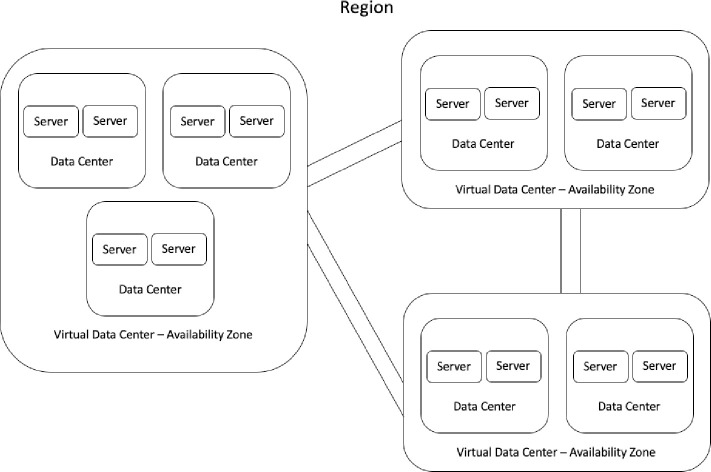
A Virtual Data Center (VDC) has at least 2 physical data centers composed by 2 server nodes.
A combination of 3 or more VDC’s is a geographic Region.
The components of a DS are located in many different machines over a network. The communication and orchestration of process are done by sending and receiving messages. The service exposed are defined by the aggregation of components and its interactions provide the software functionality. Systems such as Service-Oriented Architecture (SOA), peer-to-peer(P2P) and Micro-Services are examples of distributed applications.
Deploying and synchronizing components over many distributed cluster of nodes can be very complex due to multiple variables that can affect the quality of the solution such as network latency between data centers at business hours and at on-demand; cost of renting machines from different Computing Providers; shared servers resources utilization (“noisy neighbor effect”- at both virtual machines and bare metal); valorization of the dollar due to macro and micro economics factors; change in processing time due to model of nodes available for a given time period and operating complexity of the technology stack.
There are many algorithms proposed in the literature to solve the routing-scheduling problem such as 2opt, ant colony (AC), greedy algorithm, genetic algorithm (GA), neural networks, Cross Entropy, and simulated annealing (SA) but very limited work is found using Algorithmic Information Theory to find the boundaries of decision problems in Turing Machines. In this paper we propose a variation of the TSP by defining the decision problem for the candidate solution as a Shannon-Bernoulli process that follows a log-normal distribution for the cost distance variable, defined as a dependable utility function for the TSP.
An orchestration job has to deploy efficiently S types of services, process or tasks in many different computing resources such as a cluster of containers or a pool of (physical or virtual) machine nodes connected over a distributed network with different weights (or costs) between each pair of nodes. This job is a process that needs to run on all M (unique) resources points. The cost to use each node can be defined as the round-trip latency between the nodes in the network or the financial cost associated to the proportional quantitative utilization rate for each resource in a given time period. As more Computational Capacity is added, choosing the shortest route to multiple target nodes will be more computationally complex. Fig 2 illustrate a service orchestration across a set of distributed clusters of machines connected over a common network.
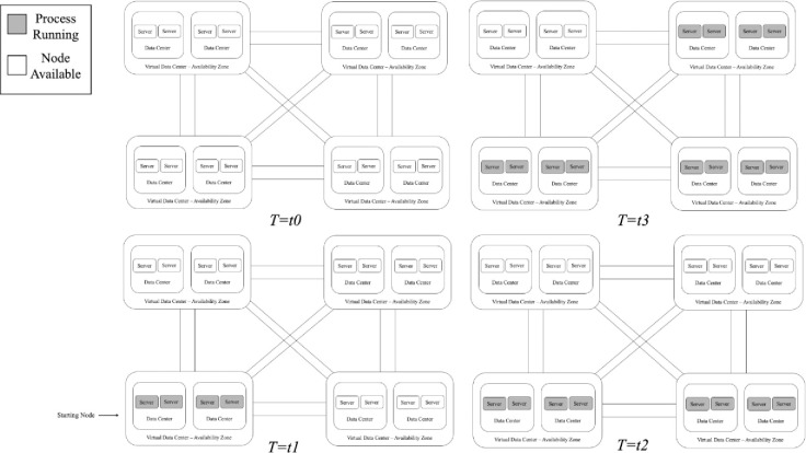
Computing provider’s distributed over a network of machines with the respective published service’s and available nodes.
Materials and methods
The traveling salesman problem
was introduced by William Hamilton and Thomas Kirkman. It also known as the messenger problem. The problem asks given a list of cities and the distance between each pair of nodes what is the shortest route that visits all cities exactly once and returns to the original city at the end. There are several researches dedicated to address this routing problem and it has applications in mathematics, computer science, statistics and logistics.
The computational complexity of an algorithm shows how much resources are required to apply an algorithm such as how much time and memory are required by a Turing machine to complete execution and can be interpreted as a measure of difficulty of computing functions. A measurement of computation complexity is the big O notation. It can be defined as: Let two functions f and g such as f(n) is O(g(n)) if there are positive numbers c and N such that

The TSP problem is an important combinatorial optimization problem. As most of the decision problems, it is in the class of NP-hard problems.
Consider a salesman traveling from city to city and some of them are connected. His goal is to visit each city exactly once and go back to the first city when he finishes. The salesman can choose any path as long as its valid (i.e. visit each city once and finish at the city it has started the tour) he also wants to minimize his cost by taking the shortest route. This problem can be described as a weighted graph G where each city is a node (or vertex) and is connected by a weighted edge only if the two cities are connected by any kind of road, and this road do not cross any other city. The utility function in the TSP is the Euclidian distance. Fig 3 demonstrate the cost matrix between each pair of nodes of a set defined by valid (non-repeating) permutations in a language L with symbols {A, B, C, D}. The cost/weight between points is calculated as a Euclidian distance in a 2D graph.
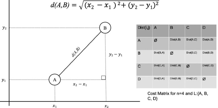
A sample cost matrix for 4 nodes and the Euclidian distance between each pair of nodes.
Table 1 Demonstrate a sample of valid and invalid strings created from L.

| Word w in Language L | Path Sequence for L: {A, B, C, D, E} | Is Hamiltonian? |
|---|---|---|
| Valid | A > B > C > D > E > A | Yes |
| Valid | D > B > C > A > E > D | Yes |
| Valid | D > B > A > C > E > D | Yes |
| Invalid | A > B > A > D > E > A | No |
The graph can be represented as a matrix where each cell value is defined as the respective cost (distance) w between nodes v and u. For N nodes the distance matrix is defined as D = w(v,u) for all (unique) pair of N. The goal of the TSP is to find a permutation π that minimizes the distance between nodes. For symmetric instances the distance between two nodes in the graph is the same in each direction, forming an undirected graph. For asymmetric instances the weights for the edges between nodes can be dynamic or non-existent.
The weigh value of the edge is defined as the distance of the tour (roads) between cities.
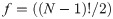
For symmetric TSP, as the number of nodes (or cities) increases in the graph G, the number of possible tours growth choice also increase and is factorial. If we consider N nodes, the function of the input size is
Computational complexity theory
Problems in the NP class can be solved by a non-deterministic polynomial algorithm. Any given class of algorithms such as P, NP, coNP, regular etc. must have a lower bound that index the best performance any problem in the class can have. This bound can be described as the total amount of input items (or symbols) a machine must process before halting, and the respective output items produced following a Probability Distribution Function and a given finite Alphabet. A strategy to find a solution to the decision problem is to find a function that reduce or transform a problem from a domain in which there is no know solution to a constrained domain with a known solution.
This allows the algorithm to search the solution space and decide if any solution is a valid (yes-instances) or invalid (no-instances) and its computable by a polynomial-time algorithm.
This strategy allows us to map instances of the Hamiltonian circle problem to a decision version of the Traveling Salesman Problem and can be described as a decision problem to determine if exists a Hamiltonian circuit in a given complete graph with positive integer weights hose length is not greater than a given positive integer m. Each valid (yes-instance) in the TSP problem is mapped to a valid instance in the Hamiltonian problem space and this transformation can be done in polynomial time.
In Fig 4 reproduced from [2] we have a visual representation of computational complexities categories. The figure demonstrates the groups of Regular, P, coNP, NP, etc class of recognizable problems. In complexity theory, the class P contains all decision problems solvable by a deterministic Turing Machine in polynomial time. The Nondeterministic Polynomial time (NP) class of problems is a category of decision problems that is solvable in polynomial time by a non-deterministic Turing Machine.
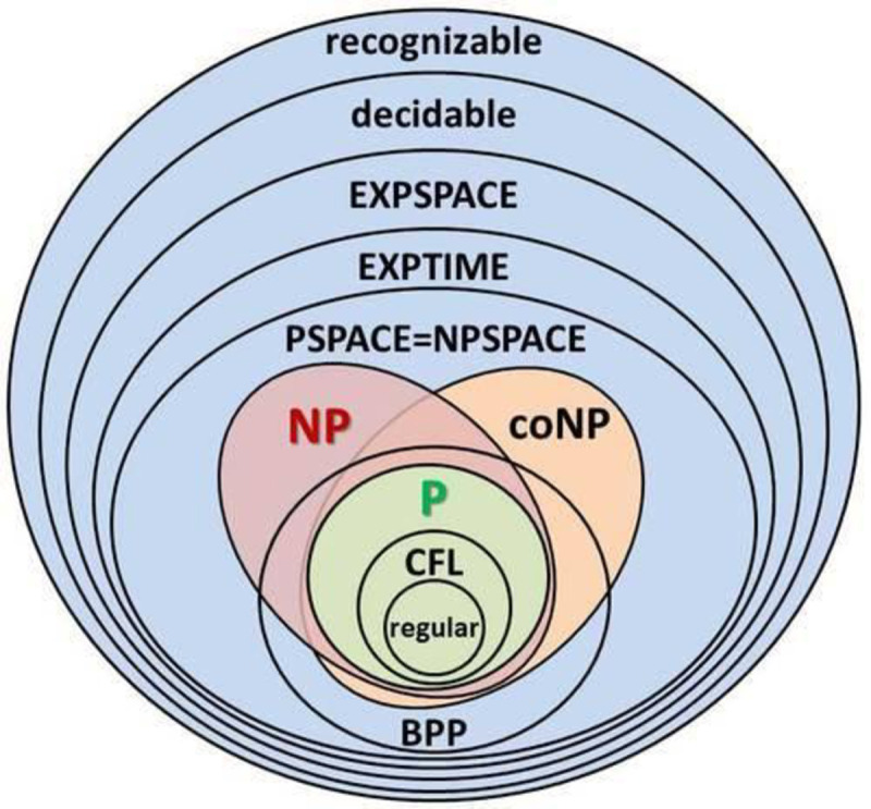
Diagram representation for the many categories of computational complexity.
The coNP are the class of problems that have a polynomial-time algorithm mapping for “no-instance” solutions which can be used to verify that the proposed solution is valid but there is no such mapping for “yes-instances”. The P class is a subset of both coNP and NP. The bounded-error probabilistic polynomial time (BPP) is a class of problems solved by a probabilistic Turing Machine in polynomial time with an attached probability distribution function with a given error degree. BPP can be interpreted as the complexity class P with a randomness boundary factor.
Hamiltonian graph
A Hamiltonian cycle (or circuit) can described as a "path" that contains all nodes and the elements in this set are not repeated, with exception to the final vertex. This means that a Hamiltonian cycle in G with start node v has all other nodes exactly once and them finishes at node v. A graph G is Hamiltonian if it has a Hamiltonian cycle. A Hamiltonian cycle with minimum weight is an optimal circuit and therefore is the shortest tour in the TSP Problem.
The Fig 5 provides an example of Hamiltonian circuit for a Graph G with 5 nodes {A, B, C, D, E}. The Table 2 shows the cost matrix for the super graph G.
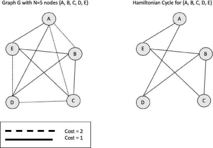
Hamiltonian cycle from a super graph.
| Cost Matrix | A | B | C | D | E |
|---|---|---|---|---|---|
| A | 0 | 2 | 2 | 1 | 1 |
| B | 2 | 0 | 1 | 1 | 1 |
| C | 2 | 1 | 0 | 2 | 1 |
| D | 1 | 1 | 2 | 0 | 2 |
| E | 1 | 1 | 1 | 2 | 0 |
Although heuristics methods define special cases for the TSP problem and produces near-optimal solutions with short length (weight) Hamiltonian cycles it does not guarantee that the results are the shortest circuit possible. The algorithms to solve the TSP are grouped in 2 categories: exact (Brute-force, greedy) and approximation algorithms (Heuristics such as Simulated Annealing and Genetic Algorithm).
Nature inspired models
Researchers have proposed algorithms inspired by natural events and structures like the heating of metals and the growing behavior of biological organisms. Those methods do not iterate over the entire solution space but rather a portion in order to find the local minimum. They start with an initial random solution and tries to improve the solution quality over each interaction until some input Threshold parameter factor T is reached like a maximum number of interactions; maximum number of candidate solutions; no further improvements found after several iterations; the rate of decay in a dependable temperature probabilistic function or a minimum quality threshold is achieved.
Therefore, heuristics approximation methods can be interpreted as a non-deterministic way to address the error rate between the known solutions and the unknown solutions in polynomial time (i.e. Entropy reduction methods). Although such algorithms do not have to traverse the entire solution space it must decide–“outguess” or “bet”—when a random candidate solution with negative gain will be accepted (i.e. candidate with worst solution quality than current know best solution) in the hopes that eventually it would lead to the shortest distance (i.e. a better solution quality).
Nature-inspired models such as Genetic Algorithms (GA), Ant Colony (AC) and Simulated Annealing (SA) use prior information to improve the solution results and thus are biased towards this encoding. Alternatively, by modeling the TSP problem as a communication channel with a probability density function associated with the stochastic process that generates the solutions at random (following a Bernoulli process), thus we can bound the limits of the search space to a log-normal distribution.
The advantage of this method is that by relying on the statistical analysis of the solution space instead of the computational complexity of the problem we can have equal or better quality than the traditional algorithms without relying on computationally complex implementations that have a higher time and space constrains.
Therefore, this paper attempts to provide an algorithm to solve the TSP using for the decision rule the entropy measured for the solution cost distribution H(X) and by maximizing the expected value of the logarithm of cost/weight/distance variable, defined as the utility function g(X). This is equivalent to maximize the expected geometric growth rate.
Literature review
Solving hard problems
There are 3 categories of algorithms to solve NP-hard problems such as the TSP:
Exact Algorithms: Fast to converge to a solution only form small instances of the problem.
Heuristic Algorithms: Compromise quality but converge with acceptable time requirements. Produce sub-optimal results.
Special cases: Restrict the boundaries of the solution space domain to a subproblem for which there is an exact (or better) solution quality.
Exact Algorithms try all permutations in the domain and verify if each candidate string is the best solution. This algorithm uses a brute-force search method. The running time has a computational complexity of O(n!). As the number of nodes increases the complexity (or running time) increases with a factorial growth.
Combinatorial problems
Other approaches such as Branch and bound algorithms can be used to optimize combinatorial problems. The branch-and-bound method produces lists of candidate solutions by a search in the state space. The set of states forms a graph. Each sub pair of states is connected if the first and the second state are produced by an operator to transform the first state in the second state.
From Poole and Mackworth [3], there are two categories of state space search algorithms:
Uninformed: The algorithm does not have any prior information about the state distribution. The Breadth-First Search is an instance of this class.
Heuristic Search: The algorithm has encoded information about the solution distribution defined by a heuristic function. The A* search algorithm is an instance of this class. The A* is a path finding algorithm and its defined in terms of weighted graphs. It has a running time of O(bd).
Heuristic algorithms
are method for problem-solving using approximations to find suboptimal solutions, under some predefined degree of freedom. There are many heuristics designed to address the TSP as a combinatorial optimization such as genetic algorithms, simulated annealing, tabu search, ant colony optimization, swarm intelligence and cross-entropy method. There are two class of heuristics: Constructive Methods and Iterative Improvement.
Constructive heuristics
Starts with an empty solution and expands the current know partial solution at each execution time unit until the target complete solution is found. In the Nearest neighbor (NN) algorithm, the salesman starts at a random city and at each execution time it visits the nearest city (performing a local move) until all nodes have been visited. The method can be optimized by pre-processing (or filtering) the possible candidate solutions to clusters of best-quality arrangements of node distributions in a 2D graph. This optimization method works as a prefix code property. The method has a worst-case performance of O(N2).
Nearest Neighbor (NN) and Nearest Insertion (NI)
From Asani, Okeyinka and Adebiyi [4] the Convex-hull and Nearest Neighbor heuristics can be combined. Their results where compared with two benchmark algorithms Nearest Neighbor (NN) and Nearest Insertion (NI). Their experimental results show their approach produces better quality in terms of computation speed and shortest distance.
The Christofides and Serdyukov algorithm
Based in graph theory and combines a minimum spanning tree with a minimum-weight perfect matching where the distances between nodes in a super-graph is symmetric and follow the triangle inequality and thus form a metric space. The solution Christofides algorithm has the best worst-case scenario currently know with a quality tour of at most 1.5 the optimal string. The computational complexity is O(n3).
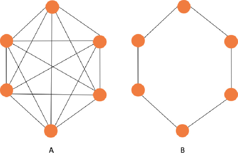
Given a Eulerian path we can find a Eulerian tour in O(n) time. The method finds a minimum spanning tree and duplicate all edges to create a Eulerian Graph. A graph G = (V(G), E(G)) is Eulerian if is both connected and has a closed trail and thus represents a tour with no repeated edges, containing all edges of the graph. In graph theory a Eulerian path is a string in a finite graph that visits every edge exactly once (no repeated edges) and it allows the revisiting of nodes, then returning to the starting vertex. In Fig 6 we have a comparison between Hamiltonian and Eulerian graphs.
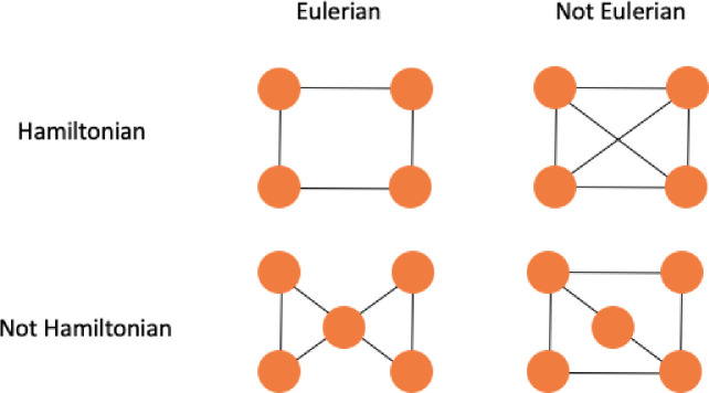
Example of Hamiltonian and Eulerian graphs.
The Christofides and Serdyukov algorithm can be described as:
Find the minimum spanning tree
Create a map for the problem with the set of nodes of odd order
Find a Eulerian tour path for the map
Convert to the TSP: If a node is visited twice create a shortcut from the node before the current and next node.
Iterative improvement
Algorithms such as the Pairwise exchange method implemented by the 2-opt algorithm remove two edges at each interaction and reconnected the edges by a new shorter path.
k-opt method
The 2-opt and 3-opt are a special case of the k-opt method. The method can be optimized by a preprocessing using the greedy algorithm. For a random input the average running time complexity is O (n log(n)).
2opt, k-opt
Croes proposed the 2-opt algorithm [5], a simple local-search heuristic, to solve the optimization problem for the TSP. It works by removing two edges from the tour and reconnects the two paths created. The new path is a valid tour since there is only one way to reconnect the paths. The algorithm continues removing and reconnecting until no further improvements can be found. k-opt implementations are instances of 2-opt function but with k > 2 and can lead to small improvements in solution quality. However, as k increases so does the time to complete execution.
In his work [6] proposed the Tabu Search method and it can be used to improve the performance of several local-search heuristics such as 2opt. As neighborhood searches algorithms like 2opt can sometimes converge to a local optimum, the Tabu search keeps a list of illegal moves to prevent solutions that provide negative gain to be chosen frequently. In 2opt the two edges removed are inserted in the Tabu list. If the same pair of edges are created again by the 2opt move, they are considered Tabu. The pair is kept in the list until its pruned or it improves the best tour. However, using Tabu searches increases computational complexity to O(n3), as additional computation is required to insert and evaluate the elements in the list.
The Fig 7 show the 2-opt moves from [7].
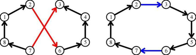
Generating 2-opt moves.
[8] compared several heuristic strategies for the TSP problem such as Greedy, Insertion, SA, GA, etc. He investigated the performance tradeoff between solution quality and computational time. He classifies the heuristics in two class: Tour construction algorithms and Tour Improvement algorithms. All algorithms in the first group stops when a solution is found such as brute-force and Greedy Algorithm. In the second group, after a solution is found by some heuristics, it tries to improve that solution (up to a certain computation and/or time constraints) such as implemented by 2opt, Genetic Algorithm and Simulated Annealing. He concluded by showing that the computational time required is proportional to the desired solution quality.
Simulated Annealing (SA)
Simulated Annealing are heuristics with explicit rules to avoid local minimal. It can be described as a local random search that temporarily accepts moves with negative gain (i.e. were produced by solutions with worst quality than current). These methods simulate the behavior of the cooling process of metals into a minimum energy crystalline structure.
This concept is analogous to the search of global maximum and minimum. The probability of accepting a solution is set by a dependable probability function of a temperature parameter variable t. As the temperature decreases over time the probability changes accordingly. Fig 8 demonstrates the simulated decay in the temperature function over the number of interactions in an algorithm.
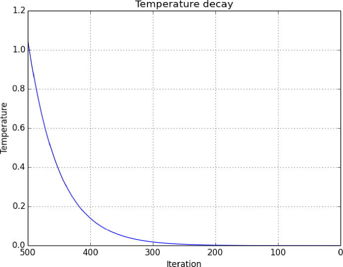
Temperature decay relative to the iterations of the SA algorithm.
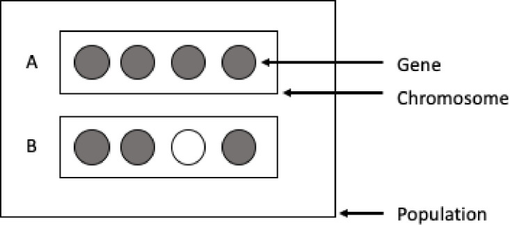
The acceptance probability is defined as p(x) = 1 if f (y) ≤ f (x) and when otherwise
[9] research combines the Simulated Annealing method with the Gene Expression Programing to improve solution diversification and state search. Their results show a better performance that other methods such as ant-colony, naive SA, naive GA, etc.
The SA algorithm specifies the neighborhood structure and the cooling function.
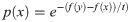
Fig 9 from [9] represents the SA algorithm flowchart.
Simulated annealing algorithm flowchart.
[10] research explores the optimization technique in Simulated Annealing and the solution impact by different temperature schedule designs. It concludes that the quality of finite time SA implementations is a result of relaxations dynamics similar to the analogy with the vitrification process of amorphous materials (non-crystalline) or disordered systems (high entropy).
Their results can be generalized in terms of entropy distributions. By the thermodynamics analogy, we know the position of particles in higher temperatures have a higher degree of uncertainty and thus there is more entropy as each particle is bouncing randomly. As the temperature decreases the particles forms bounds between them and the overall state distribution forms a glassy or crystal structure. As there is less uncertainty about the average state value for each particle there is less entropy and thus more information about the optimal state distribution is known.
[11] work provide a numerical analysis of the simulated annealing applied to the TSP. The cost distribution is compared to the control parameter of the cooling method. It concludes that the average-case performance can be defined by assuming the deviation between the final total cost and the optimal solution is distributed by a gamma distribution. This behavior is also observed in our research and this model is explained by the Kolmogorov Complexity for the Bernoulli string that represents a random solution candidate. The entropy for this distribution can be calculated and is the maximum entropy probability distribution. This is the sufficient statistics needed to represent the state set.
Metropolis algorithm and heuristic optimizations
Let f(X) be a function with output proportional to a given target distribution function r. The function r is the proposal density. At each iteration of the algorithm it attempts to move around the sample space. For each move it decides sometimes to accept a given random solution or stay in place. The probability of the solution of the new proposed candidate is with respect to the current know best solution. If the proposed solution is more probable than the know existing point, we automatically accept the new move. Else if the new proposed solution is less probable, we will sometimes reject the move and the more the decrease the probability, less likely we will accept the new move. Most of the values returned will be around the P(X) but eventually solutions with lower probability will be accepted. This characterizes can be interpreted as a generalization of the methods proposed by Simulated Annealing and Genetic Algorithms.
Other heuristics such as 2-opt, 3-opt, inverse, swap methods can be used to generate candidate solutions. Several researches such as [8] have been made to study the performance of different SA operators to solve the TSP problem [12]. proposed a list-based SA algorithm using a list-based cooling method to dynamically adjust the temperature decreasing rate. This adaptive approach is more robust to changes in the input parameters. Their research provide an improved Simulated Annealing method that uses a dynamic list to simplify the parameter settings. This method is used to control the cooling rate for the decrease temperature used by the Metropolis Rule. The list is updated iteratively following the solution space topology. This cooling schedule can be defined as a special geometric cooling method with variable coefficients. This characteristic gives the algorithm more resistance to different input parameters values while producing good sub-optimal results.
In his work [13] proposed a biological inspired bee system to optimize the routing in Railway systems. They conclude that the average solution results are better or equivalent than the traditional SA and GA methods.
The quality of the solution can be improved by allowing more time for the algorithm to run. [14] observed that the performance of 2-opt and 3-opt algorithms can be improved by keeping an ordered list of the closest neighbors for each city-node and thus reducing the amount of solutions to search but requiring more memory to keep the list of states.
Genetic Algorithm (GA)
Genetic Algorithms was first introduced by [15] based on natural selection theory, as a stochastic optimization method in random searches for good (near-optimal) solutions. This approach is analogous to the "survival of the fittest" principle presented by Darwin. This means that individuals that are fitter to the environment are more likely to survive and pass their genetic information features to the next generation.
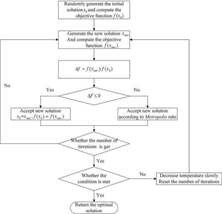
In TSP the chromosome that models a solution is represented by a "path" in the graph between cities. GA has three basic operations: Selection, Crossover and Mutation. In the Selection method the candidate individuals are chosen for the production of the next generation by following some fittest function In the TSP This function can be defined as the length (weight) of the candidate solutions tour. In Fig 10 we have a representation of genes and chromosomes.
Chromosome for a sample of individual candidate solutions.
In Fig 11 is demonstrated an example of two parents under the Mutation and Crossover operators to generate a new offspring.
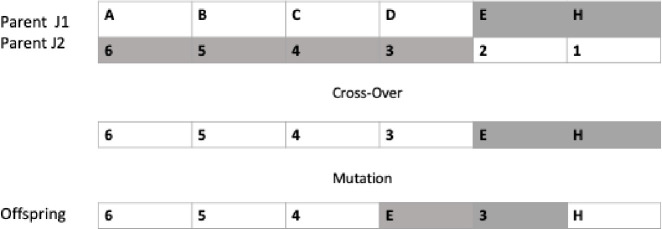
Offspring representation for the genetic algorithm mutation and crossover operators.
Next those individuals are chosen to mate (reproduction) to produce the new offspring. Individuals that produce better solutions are more fit and therefore have more chances of having offspring. However, individuals that produces worst solutions should not be discarded since they have a probability to improve solution in the future. In other words, the heuristic accepts solutions with negative gain hoping that eventually it may lead to a better solution.
Several researches have studied the performance trade off of selection strategy and how the input parameters affect the quality of solution and the computational time [16]. in his work explores different selection strategies to solve the TSP and compare the performances quality and the number of generations required. It concludes that tournament selection is more appropriate for small instance problems and rank-based roulette wheel can be used to solve large size problems.
[17] compared the quality of the solution and the convergence time on many selection methods such as proportional, tournament and ranking. They conclude that ranking and tournament have produced better results that proportional selection, under certain conditions to convergence. In his work [18] explored proportional roulette wheel and tournament method. He concluded tournament selection is more efficient than proportional roulette selection. Their work presents a simple genetic algorithm that combines roulette wheel and tournament selection. Their results suggest that this approach converges faster than roulette wheel selection.
This conclusion is related to the findings in our research and can be explained by Information Theory. The tournament selections mechanism helps to avoid the algorithm to waste execution iterations with solutions that have more noise (i.e. local minimum candidates–suboptimal solutions) and also by providing more useful information by giving a chance for all candidate to eventually produce optimal solutions, through the roulette wheel method.
The Fig 12 contains the pseudo-code for a Genetic Algorithm from [19].
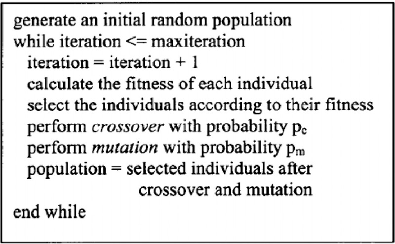
Basic genetic algorithm.
Ant Colony (AC) optimization
Ant colony (AC) optimization is a method that models the behavior of ants to find the shortest route in the nest. The choice for a given path by each ant is defined by the distribution of pheromones left by other ants when in transit.
The method is described as:
Initialize: Create initial distribution of pheromone in the region
For i from (0, n)
For each ant
Evaluate the objective function Update know best solution tour Update pheromone intensity distribution Simulate decay pheromone intensity
Stop Criterion Achieved?
Yes: Local minimum found Continue search until maximum iteration n is reached.
In the work “Ant supervised by PSO and 2-Opt algorithm, AS-PSO-2Opt, applied to Traveling Salesman Problem” from Kefi, Rokbani, Krömer and Alimi [20] there is a optimization of the 2-opt method using a post-processing for the solution paths to help avoid local minimum. Their results perform better than other benchmark algorithms such as Genetic Algorithm and Neural Networks.
In Fig 13 we have a representation of ant nest and pheromone distribution across a 2D region.
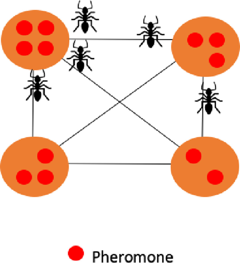
Ant colony pheromone representation.
Cross-entropy (CE) method
Is a combinatorial optimization method with noise. The method approximates the optimal utility function estimator with two targets:
Create a sample from a probability density function.
Minimize the cross-entropy between the distribution and the density function to improve the candidate solution quality for the next iteration.
The CE algorithm can be described as:
Init: Set parameter μ as average and σ as the standard deviation
For i in (0, N)
Create random sample S with size n using a normal distribution N (μ, σ) with parameters μ and σ Evaluate the Noise (entropy) distribution for the sample S Select the best Z% candidates of the solution sample to form a new subset T ⊆ S Update μ and σ with the probability distribution function of T, assuming a normal distribution
The algorithm works by reducing the entropy using a maximum like hood estimator P(X). In Fig 14 we have a representation for the entropy function P(X).
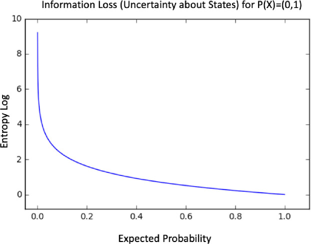
Entropy decrease process.
In “Solve Constrained Minimum Spanning Tree By cross-entropy (CE) method” [21] propose a parallel, randomized method to find a spanning tree using the lowest total cost relative to the cost weight under constrained weight boundaries.
Special cases are a class of algorithms that restricts the limits in the problem to find the optimal solution inside a give boundary. A metric TSP defines the distance between nodes under the triangle inequality and replaces the Real value Euclidian for the Manhattan distance. The Euclidian TSP is a special case for the metric TSP using integer numbers for the Euclidian distance.
The Euclidian TSP has a Euclidian minimum spanning tree associated with the minimum spanning tree of the graph and has the expected running time complexity O(n log n).
Proposed method
Background theory review
Information Theory (IT)
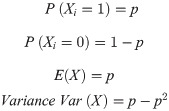
Quantifies the amount of information in a noisy communication channel and is measured in bits of entropy. IT is based in probability theory and statistical distributions. Entropy quantifies the amount of uncertainty in a random Bernoulli variable created by a Bernoulli process thus information can be interpreted as a reduction in the overall uncertainty about a set of finite states. Mutual information is a measure of common information between two random variables and it can be used to maximize the amount of information shared between encoded (sent) and decoded (received) signals. In Table 3 we have the relationship between Information and Entropy. As we increase our knowledge about the states following a probabilistic function distribution, we reduce entropy, as there is less uncertainty about possible state outcomes.
| Information | Entropy | Word | P (X = 0) | P (X = 1) | E(X) |
|---|---|---|---|---|---|
| High | Low | 0000 | 1 | 0 | 1*1*1*1 = 1 |
| Medium | Medium | 0001 | 0.75 | 0.25 | 0.75*0.75*0.75*0.25 = 0.105 |
| Low | High | 0011 | 0.5 | 0.5 | 0.5*0.5*0.5*0.5 = 0.0625 |
Information theory as an approximation method
Information Theory has applications in a range of fields and is used as a mathematical framework for encoding and decoding of information such as in adaptive systems, artificial intelligence, complex systems, network theory, coding theory, etc. IT quantifies the number of bits required to describe a given a set of states using a statistical distribution function for the input data.
Entropy of a random sequence
Entropy is a measure of uncertainty of a random variable. It is the average rate at which information is produced by a stochastic process [22]. defined the entropy H as a discrete random variable X with possible values as outcomes draw from a probability density function P(X). Fig 15 demonstrate the variation in entropy H(X) vs a Bernoulli distribution. In Eq 4 the entropy function is defined as:
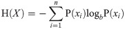
Entropy H(X) vs Probality Pr(X = 1).
Random variables and utility function
Let X be an independent random variable with alphabet L: {001, 010, 100–}. A utility function g is used to model worth or value and is defined by g: {X ⊂ ℝ} and it represents a preference of relation between states. The utility function Y = g(X) of a random variable X express the preference of a given order of possible values of X. This order can be a logical evaluation of the value against a given threshold or constant parameter. The g(X) is defined by a normal distribution with given mean and variance under some degrees of freedom (i.e. confidence level).
As an example if g(X1 = 001 = 1) = c1 and g(X2 = 010 = 2) = c2 are the costs of two routes between a set of nodes in a super-graph G*, we can use this function to determine the arithmetical and logical relationship between them and decide if c1 is worst, better, less, greater or equal to c2. Therefore g(X1) < g(X2). The probability density function pdf(Y) can be used to calculate the entropy of the distribution of the cost values. An exponential utility is a special case used to model when uncertainty (or risks) in the outcome between binary states and in this case the expected utility function is maximized depending on the degree of risk preference.
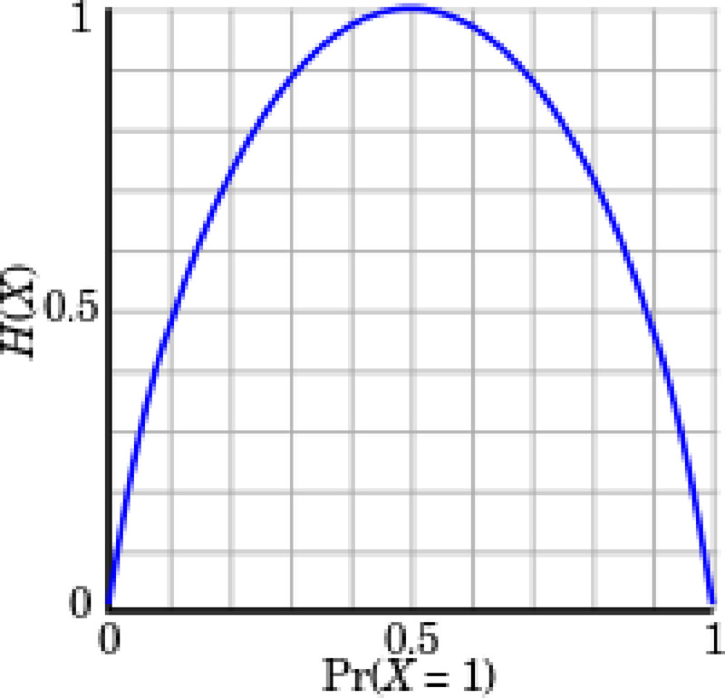
Fig 17 demonstrate an example of a normal distribution for cost function g(X) = {50, 51, 49, 49.3, 50.5, 50.3, 49.1, 48} and the probability P(X<48). Fig 16 shows the histogram for g(X). Table 4 demonstrate the calculation for the mean, standard deviation and variance for g(X), thus we have:
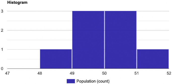
The probability density function for cost function g(X).
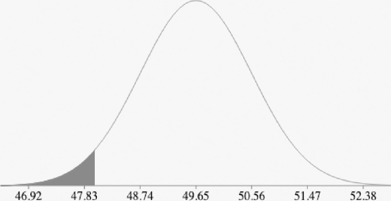
The normal distribution with mean 49.65 and standard deviation 0.91.
Then P (X<48; X < min g(X)) = 0.0349.
| Parameters | Output |
|---|---|
| Standard Deviation, σ | 0.91241437954473 |
| Count, N | 8 |
| Sum, Σx | 397.2 |
| Mean, μ | 49.65 |
| Variance, σ2 | 0.8325 |
Kolmogorov complexity
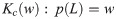
The Kolmogorov complexity [23] of a string w from language L denoted by
Complexity of a string and shortest description length
Let U be a Universal computer (i.e. Universal Turing Machine). If description d(x) is the minimal string to encode x. Kolmogorov complexity Kc(x) of a string x of a computer U is


Measuring the randomness of a string
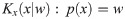
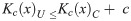
Let Kc (x|y): The conditional Kolmogorov complexity of Xn given Y. Consider for example we want to find the binary string with higher complexity between three variables X1(010101010101010), X2(0111011000101110) and Y (01110110001011). In Table 5 we have the representation and minimal encoding using Xn and Y. Therefore, we can see X1 and X2 can be encoded as combinations of Y and thus Kc(X1|Y) > Kc (X2| Y). This relationship is defined as

| Variable | Binary Sequence | Minimal String Representation Schema |
|---|---|---|
| Y | 01110110001011 | Substring |
| X1 | 010101010101010 | 01 (#7 pairs of bits) + 0 (#1 single bit) |
| X2 | 011101100010110 | Y + 0 |
In Fig 18 from [24] we can see a comparison between a series of strings and the correspondent automata state machine and the regular expression patterns (i.e. regex schema).
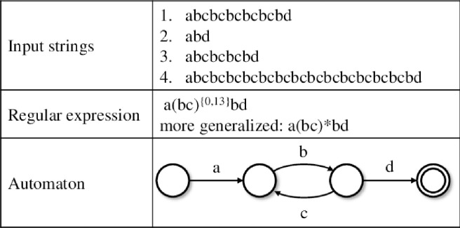
Examples of representations of a given input string set using regex and an automaton.
The expected value of the Kolmogorov complexity of a random sequence is close to the Shannon entropy. From [25] this relationship between complexity and entropy can be described as a stochastic process drawn to a i.i.d on variable X following a probability mass function pdf(x). The symbol x in variable X is defined by a finite alphabet L. This expectation is
Kelly criterion and the uncertainty in random outcomes
The Kelly strategy is a function for optimal size of an allocation in a channel. It calculates the percentage of a resource that should be allocated for a given random process. It was created by John Kelly [26] to measure signal noise in a network. The bit can be interpreted as the amount of entropy in an expected event with two possible binary state outcome and even odds. This model maximizes the expectation of the logarithm of total resource value rather than the expected improvement for the utility function from each trial, in each clock unit iteration in a Turing Machine.
The Kelly criterion has applications in gambling and investments in the securities market [27]. In those special cases, the resource (communication) channel is the gambler’s financial capital wealth and the fraction is the optimal bet size. The gambler wants to reduce the risk of ruin and maximize the growth rate of his capital. This value is found by maximizing the expected value of logarithm of wealth which is equal to maximize the expected geometric growth rate.
Similarly, the log-normal Salesman’s can improve his strategy in the long run by quantifying the total of available inside information in the channel (or a tape in the Turing machine) and maximizing the expected value of the logarithm of the value function (defined by Traveled Euclidean distance) for each execution clock. Using this approach, he can reduce his uncertainty (entropy H(X)) while optimizing his rate of distance reduction (and solution quality improvement) at each execution time.
The Fig 19 demonstrate the Kelly criterion value over the Expected Growth Rate.
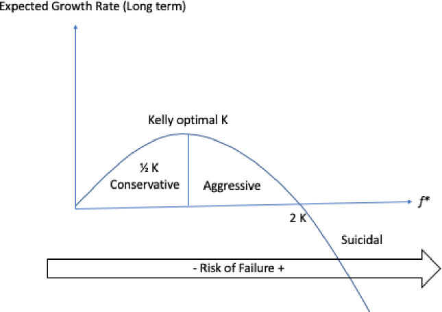
Maximization of entropy in random events.
Kelly uncertainty distribution
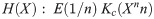
Let E(Y) be the expected value of random variable Y, H(Y) be the measured entropy for the pdf(Y) distribution and K*(E(Y),H(Y)) = f* be the maximization of the expected value of the logarithm of the entropy of the utility function Y = g(X). This fraction is known as the Kelly criterion and can be understood as the level of uncertainty about a given data distribution of the random variable X relative to a probability density function pdf(Y) of a measured respective cost distribution found at the sample. It’s a measurement of the amount of useful encoded information.
The value of f* is a fraction of the cost-value of g(X) on an outcome that occurs with probability p and odds b. Let the probability of finding a value which improves g(X) be p and in this case the resulting improvement is equal to 1 cost-unit plus the fraction f, (1+f). The probability of decreasing quality for Y is (1-p).
The maximization of the expected value f* is defined by the Kelly criterion formula in Eq 12
For example, consider a program with a 60% chance of improving the utility function g(X) thus p = 0.6 (success) and q = 0.4 (failure). Consider the program has a 1-to-1 odds of finding a sequence which improves g(X) and thus b = 1(1 quality-unit increase divided by 1 quality-unit decrease). For these parameters the program has a 20%(f* = 0.20) of certainty that the outcomes produce values that improve the expected value of g(X) over many trials.
Consider another sample case for a fair coin with probability of success (winning) P (1) = 0.5(50%) and failure(losing) P (0) = 0.5(50%). Table 6 demonstrate the amount improved (+) and worsen (-) for each scenario:
| Probability | Output | Value |
|---|---|---|
| Success (1) | Gain (True) | + 2 units |
| Failure (0) | Lose (False) | - 1 unit |
The Total Expected Outcome, Edge, is defined by:


Proposed algorithm and results
Quantitative algorithmic information Theory
The algorithm is designed to find the near optimal route in a cluster of machine-nodes before returning to the original point. This problem is a variation of TSP. Tour improvement heuristics algorithms such as 2opt and Simulated Annealing (SA) are used as a benchmark for the proposed Quantitative Algorithm (QA). 3 test cases are used to analyses the solutions generated by each algorithm. The 2opt algorithms produces solutions with smaller total distance but required more time units as the number of nodes increase. SA and QA have a maximum number of allowed interactions, but QA produces better solution quality than SA for the same time period.
The test samples are grouped in 10, 30 and 50 nodes. Each point represents a machine in a data center (i.e. computing and network provider) that can deploy a given service S. The distance cost in this case is the illustrative round-trip network and processing delay. This weight is the length of time to send a signal s*(t0) plus the time to reply acknowledging of that the signal was received with another message s*ack (t1).
To avoid bias and miss interpretation in the research, the first tour loaded in the computer memory is randomly flushed using a statistical function in Python programming language. The function swaps all elements (using a normal distribution) of the initial tour list, created after reading the list of input nodes.
The solutions found from SA and QA heuristics algorithms were analyzed for accuracy and reliability of the output. We have compared the required time and solution quality between the methods. Each algorithm was measured with a trial with sample length N = 60 for 3 test cases.
Quantitative heuristic
In Fig 20 we have the flowchart design for the Quantitative TSP Algorithm (QA). The constraints for the Kelly criterion and the Bernoulli process are presented in Figs 21 and 23. The pseudo-code for the proposed Quantitative Algorithm (QA) is describe in the Table 7.
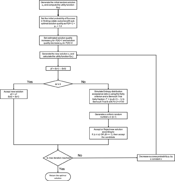
Flowchart for the Quantitative TSP algorithm based in information theory.
| Quantitative Algorithm for TSP 1. Generate the initial random solution x0 and compute the utility function f(x0) 2. Set the initial probability of Success in finding a state outcome with sub-optimal solution quality as 1. P(X = 1) = p1 = 1.0 2. and the Failure probability defined as 1. P(X = 0) = q = p0 = 1—p1 3. Set estimated solution quality increase qi for P(X) = 1 4. Set estimated solution quality decrease qd for P(X) = 0 5. Set the net fractional odds ratio as b = qi / qd 6. For i in range (0, M) 1. Generate the new solution x1 and calculate the utility function f(x1) 2. Δf = f(x1)–f(x0) 3. If Δf ≤ 0 then 1. Accept new solution 2. x0 = x1 3. f(x0) = f(x1) 4. Else 1. Simulate Entropy distribution acceptance ratio α using the Kelly criterion and a Bernoulli Trial 1. Kelly fraction α: f* = (p1(b+1)– 1)/ b 2. Bernoulli Trial B with P(1) = 1/100 to work as a random binary switch 2. Generate a uniform random number u ∈ [0,1] 3. Accept or Reject new solution according to: 1. If (u ≤ α) OR (B = = 1), then accept the candidate 1. Set x0 = x1 2. f(x0) = f(x1) 2. Else then reject the candidate solution 3. Decrease success probability p1 by a constant c 1. p1 = p1–c |
Algorithmic information model
The two major components are the simulated Kelly fraction f* (describing the overall uncertainty spread) and the Bernoulli process distribution of the underlining random event between states (estimated as the mean and standard variance for the weight function for each solution). The combination of those factors will be evaluated to decide the start of a neighborhood search (following a Probability density function) when the new alternative solution has a negative gain (i.e. new proposed solution is worse than current best-known encoded candidate).
Solutions to the TSP routing problem are explored by algorithms such as 2opt, Simulated Annealing (SA), Greedy and Genetic Algorithm (GA). In this paper we proposed a Quantitative Algorithm (QA) that does not rely on naturally inspired schemas but rather provides a statistical interpretation as a distribution of signals by a stochastic log normal process.
This stochastic process is defined as an ordered list of random variables {Xn} for a given trial of length N. N is a set of non-negative integers and Xn is defined as a target measurement for a specific instance of time.
The utility function is used to find the near optimal route that have the minimum traveling distance to multiple target node destination while returning to the starting node at the end. There are 2 constraints to be considered in the model presented in this paper: Simulated Entropy Uncertainty and Bernoulli Process.
Method Constraint 1: Entropy simulation and uncertainty measurement
Simulated Uncertainty. The first constraint is limited by the entropy. The input parameters for the Kelly function f* are the Wining probability PW and the expected net-odds b for the Bernoulli trial B. The value of PW is decreased by a fixed constant rate of 0.0001 at each interaction. The value b is measured as the ratio of average improvements of the positive interactions divided by the average reduction of the negative interactions. The result of this function is the percentage of the useful side information available in a noisy channel.
In Table 8 we have an example for the Kelly criterion calculation.
| PW (Win/Cost Decrease) | PL (Lose/Cost Increase) | Expected (Averaged) Cost Gain (Quality Improvement) | Expected (Averaged) Cost Loss (Quality Worsening) | Success/Failure Ratio b | (Output) Kelly Percentage f* |
|---|---|---|---|---|---|
| 90 | 10 | +100 | -100 | +100/|-100| = 1 | 0.8 |
| 50 | 50 | +100 | -100 | +100/|-100| = 1 | 0 |
| 10 | 90 | +100 | -100 | +100/|-100| = 1 | -0.8 |
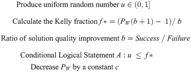
The decision criterion 1 is implemented as an evaluation of the IF logical statement for the Simulated Kelly Criterion and the Uniform Random Number output value.
Logical Statement for Method Constraint 1
For each interaction in the program
In Fig 21 we have a circuit representation of the first constraint and the representation for a sequential circuit with input and output values with a clock.
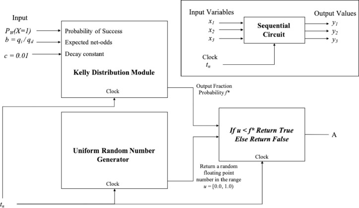
Decision Criterion 1 is implemented as an evaluation of the IF logical statement for the Simulated Kelly Criterion and the Uniform Random Number output value.
Method Constraint 2: Discrete computation distribution of a random binary variable
Bernoulli Process. The second constraint is defined by a Bernoulli process as a finite sequence of independent and random Bernoulli variables. This module will return as output the value “True” at 1% of the time for 100 interactions (N = 100) and it will accept unlikely (risky) solutions with negative gain to eventually provide improvements bets for the solution quality, under some degree of freedom. The process is defined as a trial with two binary states either “True/Success” (1) or “False/Failure” (0) with domain p ∈ [0,1]
In Fig 22 we can see a Bernoulli distribution with P (0) = 80% probability of output a Failure state
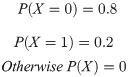
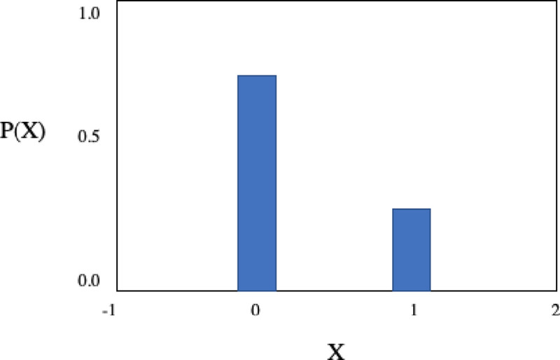
P(X) for the Bernoulli distribution with P(1) = 0.2 and P(0) = 1—P(1) = 0.8.
Examples of Bernoulli trials are show in Table 9.
| Event | Outcome |
|---|---|
| Play a game | Win/Lose |
| Coin toss | Head/Tail |
| Processing a request | On time/Late |
| Defect in equipment’s | Good/Defect |
| Buy-Sell an asset | Profit/Deficit |
| Optimizing traveling cost | Reduction/Increase |
The decision criterion 2 is implemented as a OR gate using the input Bernoulli Distribution Trial B and the output A of the IF statement from the Simulated Kelly Criterion and the Uniform Random Number output value.
Logical Statement for Method Constraint 2
For each interaction in the program
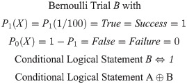
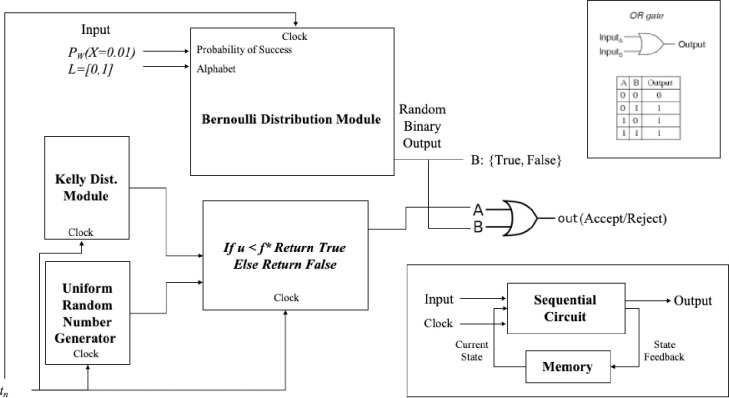
Decision Criterion 2 is implemented as a OR gate using the input bernoulli distribution Trial B and The output A of the IF statement from the Simulated Kelly Criterion and the uniform random number output value.
Algorithm analysis
This paper tries to address a few algorithm`s design questions to solve the TSP:
What is the shortest code that produces the optimal solution for the problem?
Objective: What is the minimal binary encoding, the self-information or the basic quantity required to represent the Bernoulli process
What is the path with less risk “of ruin” for the Salesman while also maximizing the solution quality?
Objective: Find the shortest Euclidian distance with less uncertainty
How to minimize running time requirements?
Objective: Optimize computational complexity
Fig 24 illustrate the TSP goal to optimize solution quality and the factors involved: Minimize Running Time; Maximize Utility Function and Minimize Code Length
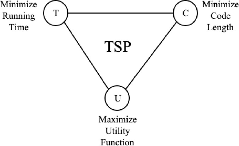
TSP target objectives.
Shortest distance and shortest encoding
The computational complexity problem in Graph Theory such as the TSP and NP-Hard Problems is reduced to a combinatorial problem, using an entropy function optimization method from a Bernoulli variable defined by a Log-Normal distribution.
The method is based on the amount of self-information available in a random variable and this is the minimum encoding required to represent the problem in a Turing Machine, while producing as output the near-optimal solution found before halting. By the Kolmogorov Complexity this is the optimal program with the minimum amount of encoded information.
Mathematical definition
Assuming the Euclidian distance between nodes is the utility function for the problem. The proposed algorithm instead of trying to find the best solution directedly, using an arbitrary stochastic process, and interactively improving the string path, alternatively, the QA algorithm assumes the symbols from output Y is produced by processing the input from Bernoulli variable X, that is defined by a log-normal distribution and variables X and Y share Mutual Information. This is the amount of information X has about Y and is equal to the information Y know about X.
The lemmas for the proposed model are defined in Table 10.
| 1. The Bernoulli process B(p) is used to generate strings with length n and a pattern-code schema encoded as a Hamilton graph with probability p 2 The strings S are a Bernoulli sequence B formed with a random variable X from a finite alphabet L 3. The utility function U(S=B(X)) = Y is defined as the Euclidian Distance between nodes in a 2D plane 4. Bernoulli variables X and Y have Mutual Information 5. The Entropy Function for H(X), H(Y) and H(X|Y) can be calculated 6. E(X) is the Expected Value for X with mean and standard deviation σ1 7. E(Y) is the Expected Value for Y with mean and standard deviation σ2 8. f*(Y) is the optimal encoding defined by the Total Expected Value (“Edge”) divided by the Expected Solution Quality Increase if Successful (“Odds”), for Sequence Y a. f*(Y) = Edge/Odds |
Logarithm utility model
The method provides an alternative narrative for the Traveling Salesman Problem as it asks, “what is the best path between cities that simultaneously minimizes cost losses in the long run while also provide the best rate of improvement for each interaction”. The salesman wants to avoid solutions with local minima. There are several possible paths the salesman can choose, and he must guess which choice will lead to the best route over a set of candidate solutions. The uncertainty between states outcomes indicates the level of entropy (i.e. more entropy means less knowledge about the state values distribution). The reverse of entropy is the negentropy, which is defined as a temporary state condition in which a certain state distribution is more probable and more organized and thus there is less uncertainty about the state distribution for a given time frame. The utility function is demonstrated in Fig 25.
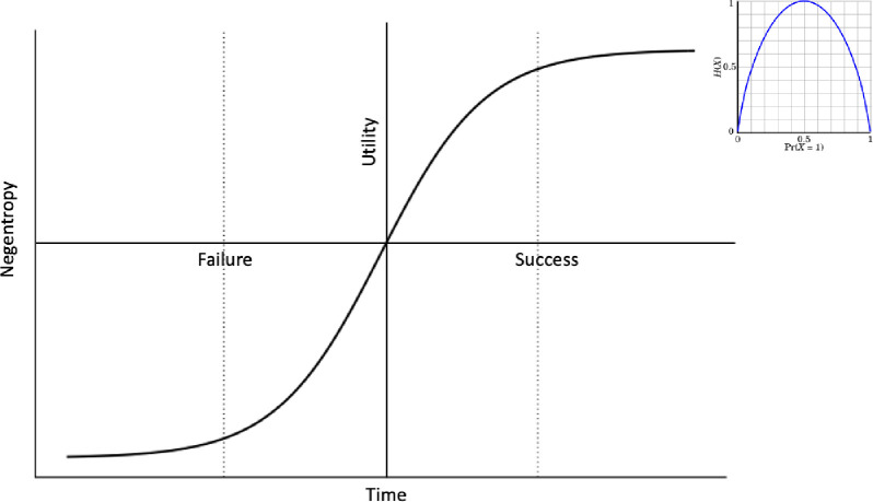
Utility function.
This approach is a model for risk measurement over many possible outcomes and is based in the work of John Kelly, Edward O. Thorp, von Neumann and Claude Shannon in logarithmic information utility, with applications in the financial markets and game theory such as the optimization in wealth growth in the long run and diversification in investment strategies in portfolio management.
Random path construction
In Fig 26 we have a representation of the possible path choices to produce a candidate solution tour for TSP. The example has an alphabet L with 4 elements (n = 4). At each interaction the Salesman’s needs to choose the next node in the route. In the begging at T = t0, starting in the arbitrary node L: {a}, it has several possibilities for the next move with L’: {b,c,d}. Each element (or symbol) has a 1/3 probability in t0. In the second iteration t1, the probability for the remaining possible symbol increase to 0.5, however the probability for the nodes already chosen drops to zero, and the possible choice outcome for the next state move is reduced to L’: {c,d}.
![Tour construction for a weighted graph with a probability function p ∈ [0,1].](/dataresources/secured/content-1765739701756-33578643-e990-416b-a955-4a9bf198ffbe/assets/pone.0242285.g026.jpg)
Tour construction for a weighted graph with a probability function p ∈ [0,1].
From initial solution in time T = t0 there are a few valid sequences that can be chosen. There is no universal function to guide the Salesman with certainty on what is the best choice. This statement is supported by the Kolmogorov complexity of the string. The Salesman must then outguess this problem using the available side-information.
The side-information can be defined by the probability density function of the Euclidian distance distribution, formed by a set of valid candidate solution strings. The condition for a candidate to be valid is to be a Hamiltonian graph. Invalid solutions have zero probability of being chosen. In Fig 27 we have a set of candidate solutions with examples of valid and invalid sequences.
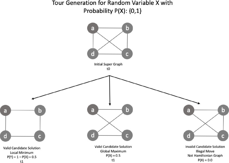
Candidate solution production and path decision.
This feature reduces the search space to only Hamiltonian circuits. From observation, we know that there is a greater probability that edges that crosses generally produce a total path distance larger than those nodes that do not have edges that overlap. The Fig 28 demonstrate a crossing of edges in a graph.
Edge crossing between nodes.
Algorithms such as 2opt takes advantage of this cluster aggrupation of edges and uses a strategy to remove the crossing between a group of nodes until no further improvement is found.
Solution quality and time to convergence
The method proposed is not an exact method but is guaranteed to produce the best quality in the long run, eventually, with probability 1 and smaller time to convergence, in average. This is a method that almost surely converges to a better solution quality if compared to any other heuristics when approaching the limit, as the number of algorithm iteration goes to infinity, and without needing complex string and array manipulations. Therefore, the method has a better computational cost optimization in average.
The proposed algorithm also brings more simplicity of implementation with lower encoding overhead, when compared to other algorithms such as Genetic Algorithm, Neural Networks and Ant Colony.
Computational requirements and cost effectiveness
The time constraining in QA heuristic is not a problem because the only factor to decide the running time is the degree of freedom allowed to the program. If the algorithm is expected to be more precise and with less errors, the time parameters can be adjusted with time complexity O(n) and with each interaction the entropy about the solution states is reduced, as the knowledge about the best solution increases (i.e. Smaller Euclidian distance). Therefore, the error rate can be adjusted to any level desired.
Relation with other heuristic methods
This is similar to the approach proposed by the Cross-Entropy Method, but the Quantitative Algorithm method does not resample or update the probability density function at each interaction, but instead embraces randomness and accepts candidate solution according to a simulated decreasing entropy function, with a binary random switch attached.
This mechanism is similar to the Manhattan Rule used by the Simulated Annealing algorithm. The proposed method use the simulated Kelly function ratio value α = f* to compare against a random control value u, than the output is evaluated again using a binary operation switch B which returns True or False, following a dependable probability function, that is decremented by a constant rate c from P(X) = 100 until P(X) = 1/100, at each interaction tN. This schema is used to provide alternatives paths and solve the hill-climbing limitation that is also present in many solvers of the TSP.
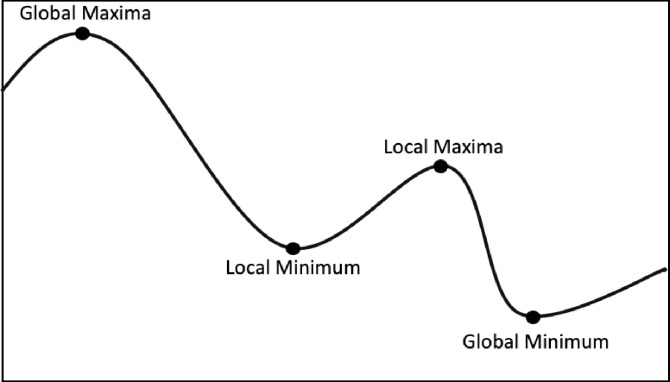
In Fig 29 we have a demonstration for the hill-climbing with examples of Global and Local points with the respective Maximum and Minimum positions.

Hill-Climbing problem.
Running costs
The running cost for the Quantitative Algorithm is the defined by the computational effort to generate a random candidate tour string and to evaluated with the current registered best-known solution, encoded by a Hamiltonian graph pattern, in O(N) time.
For each iteration, it has the computing cost to calculate the simulated entropy heuristic function and compare against the control values. These values can be calculated in constant time T(n). The memory required is defined by an array M of candidate solutions elements with size O(M) = 2. The array is a buffer to store the best candidate solution and the alternative solution.
Disadvantages and Limitations
Because of this design, the running time to converge is worst for the QA algorithm when compared to other methods, such as 2opt and greedy, at small instances of the problem with less than a few nodes (n<15). If compared to heuristics such as Simulated Annealing, Genetic Algorithm or Ant Colony the execution time is similar but requires less time in average. This behavior is observed in our computer simulation.
This is explained by the overhead in calculating the probabilistic temperature-function in Simulated Annealing (or the mutate-reproduce-selection operations in Genetic Algorithms) that are used as the acceptance criteria for the random candidate solutions and therefore the proposed entropy derived function in QA has a smaller running time overhead.
The running time cost for the proposed algorithm scales linearly to input with length n and the solution can be found in polynomial time in any Turing Machine. In Table 11 we have a comparison between classes of computational time complexity.
| Runtime Complexity | Computational Class | Time to Convergence (1/8) | Solution (Search)Space Volume | Example Algorithm |
|---|---|---|---|---|
| O(1) | Constant | 0000000000 | 0000000000 | |
| O(log n) | Logarithmic | 0000000001 | 0000000001 | Binary Search |
| O(n) | Linear | 0000000011 | 0000000011 | Linear Search |
| O(n log n) | Linearithmic time | 0000000111 | 0000000111 | k-opt method |
| O(n2) | Quadratic | 0000001111 | 0000001111 | Nearest neighbor (NN) |
| O(n3) | Cubic | 0000011111 | 0000011111 | Christofides and Serdyukov |
| O(nk) | Polynomial | 0000111111 | 0000111111 | A* |
| O(2n) | Exponential | 0001111111 | 0001111111 | |
| O(n!) | Factorial | 0011111111 | 0011111111 | Brute-Force |
| O(inf) | Infinite Time | 0111111111 | 0111111111 |
The proposed method has limitations. It needs a larger running time to converge for small instances if compared to heuristics such as 2opt and Greedy Algorithm, as it must run until the predefined max number of interactions parameter value is reached.
We have also observed that the local search methods such as 2opt, converge with less running time when the input is pre-sorted and thus help avoiding the algorithm to being lock down in local minima solutions. However, this implies that a predefined prefix schema must be directly encoded in the input string values, with the goal to improve running time performance. The pre-processing of the input string works as a prefix set for filtering “above average” solutions. This is explained by the Kolmogorov randomness of a string.
Alternatively, the proposed method does not need such implementation bias. This behavior can be explained by Algorithm Information Theory. The 2opt method for example is sensitive to the initial solution set sequence and if provided with an initial state with more noise than the running time also increases.
This means there are more elements to verify in the search space and thus more time is needed until converge. In the other hand, if there is less noise in the initial state, than the sub-optimal end state is found quickly. In comparison the proposed model is resistant to variations in the initial path sequence positions.
Computational results
The research evaluates the performance of the proposed algorithm through a series of test cases and statistical analysis. The new method is tested against the traditional method Simulated Annealing (Benchmark). Each test case was run for a trial with population length of N = 60. In the statistical analysis section, the t-test was used to compare the means between the sample groups. The null hypothesis is that there is no difference between the means of the two populations.
The input parameters where tested with different values in order to verify if the method was sensitive to changes in the controlling parameters. In the numerical simulation we have implemented 3 variations for graphs with 20, 30 and 50 nodes. Each 2D graph was used as input for the Quantitative Algorithm (QA) and the benchmark heuristic algorithm Simulated Annealing (SA). The maximum number of interactions was set to be the same with 40,000 interactions.
Similarly, to heuristics such as GA, SA and AC the method runs until it reaches a maximum number of iterations. We have set this parameter equality between the proposed and benchmark method to a fixed value of i = 40,000 iterations. The constant decay rate for the simulated entropy probability was set to c = 0.0001, the starting probability was set to p = 0.999 and variable net-odds b was defined by a random uniform value between (0.01, 2]. These parameters can be adjusted to improve the quality according to the number of input nodes, but the simulation results support the thesis the proposed method is resistant to variations in the input parameters under a given degree of freedom.
The sample trial length was also set equality to both samples with N = 60. We have also performed the Shapiro-Wilk test for normality to guarantee the input sequences were not skewed or distorted to any side. The T-Test was used to than verify if the results where statically significant in regards of the final best cost distance and the running time variables, with a confidence level of 95%.
We have also taken additional precautious to compare the performance in the numerical simulation. To achieve this all starting paths are randomly flushed—with a function in Python programing language—before execution begin, in order to guarantee the fairness when running and comparing all algorithms.
Computational statistical analysis
To demonstrate the significance and accuracy of the results we have performed a series of statistical tests to guarantee they are fair. For the numerical simulations we have created 3 test cases with 2D graphs n = {20, 30 50} nodes. Each trial has a sample with length N = 60. There are three variables recorded:
Initial Random Tour Cost: Starting total Euclidian cost for the initial path
Best Tour Cost Found: Distance for the best candidate solution found
Total Execution Time: Running Time until convergence.
The method has a few requirements:
The cost distance X can be calculated by a logarithmic utility function U
X is a random variable defined by U(X) = Y
Variables X and Y have Mutual Information
Variable X is encoded by a log-normal distribution
A path is a random sequence produced by a Bernoulli process B with probability p
The paths are Hamiltonian
The estimated value for Y is the expected solution quality
We will use a subset with N = 10 from trial with n = 50 nodes and length N = 60 to demonstrate the simulation results in Table 12.
| 50-node | ||||||
|---|---|---|---|---|---|---|
| Trial N = 60 | Initial Random Tour Cost | Best Tour Cost Found | Total Execution Time | |||
| 0 | QA | SA | QA | SA | QA | SA |
| 1 | 4584.994704 | 4350.530615 | 783.6135781 | 1013.45381 | 91.94147284 | 127.121441 |
| 2 | 4931.04388 | 3829.72755 | 1002.266343 | 856.714194 | 79.49352819 | 93.1328427 |
| 3 | 4459.545641 | 4285.493079 | 892.4679561 | 878.335327 | 67.90769484 | 73.4395111 |
| 4 | 5189.508014 | 4873.122362 | 825.1186081 | 986.814761 | 65.57152077 | 74.8066559 |
| 5 | 5303.265261 | 5389.224823 | 846.448402 | 1085.77975 | 65.92321619 | 72.4844698 |
| 6 | 4792.633045 | 4595.016823 | 1036.163983 | 855.195737 | 71.40535116 | 70.3046693 |
| 7 | 4951.587728 | 4711.457297 | 735.82339 | 1110.36984 | 61.43196151 | 78.8009844 |
| 8 | 5127.650419 | 4851.865628 | 1028.714485 | 974.535522 | 67.16026587 | 80.7510912 |
| 9 | 4213.123791 | 4227.131367 | 1006.163651 | 693.015657 | 61.80173641 | 75.0614487 |
| 10 | 4388.805181 | 5361.415343 | 887.0345646 | 813.130685 | 68.36587932 | 73.5915055 |
Fair run and descriptive statistics
We have implemented the proposed quantitative algorithm (QA) and the Simulated Annealing (SA) heuristic in a set of trials with n = {20, 30, 50} nodes and a sample with length N = 60. To guarantee the results are fair we have analyzed the distribution with the Shapiro-Wilk test to demonstrate the sample is normally distributed. The QA and SA tests for n = 50 nodes is described below:
Results from QA simulation: Initial random tour cost variable
The statistical description for the QA method distribution with n = 50 nodes and length N = 60 is described as follow
Nodes in the graph (n): 50
Sample size (N): 60
Average (): 4679.279218
Median: 4633.623941
Sample Standard Deviation (σ): 348.057997
Sum of Squares: 7147517.782
b: 2640.163152
Skewness: 0.543901
Skewness Shape: Potentially Symmetrical (pval = 0.078)
Excess kurtosis: 0.152926
Tails Shape: Potentially Mesokurtic, normal like tails (pval = 0.802)
P-value: 0.260661
Outliers: 5651.239742
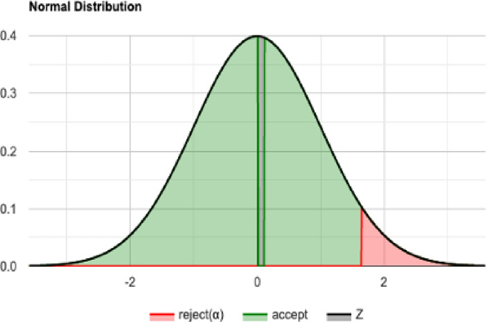
The normal distribution with average = 4679.279 and standard deviation σ = 348.057 with Significance level (α): 0.05 is shown in Fig 30. The Histogram and QQ-Plot are represented in Figs 31 and 32, respectively.
QA sample: Normal distribution for n = 50 and N = 60.
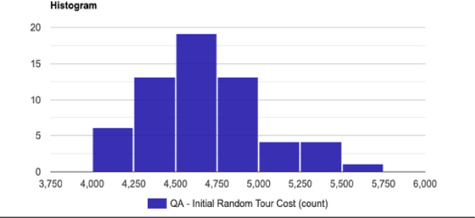
Histogram for the initial tour cost in the QA method.
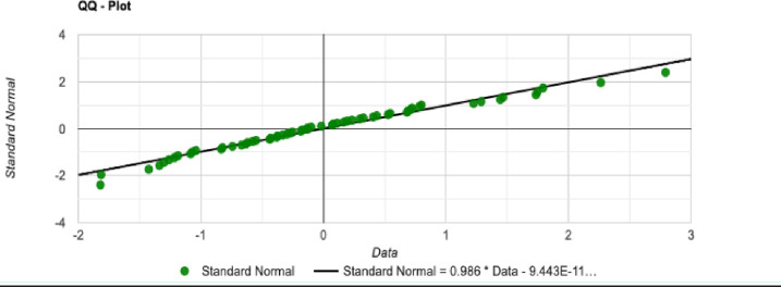
QQ-Plot for the initial tour cost in the QA method.
Shapiro-Wilk test, using a right-tailed normal distribution
H0 hypothesis
Since p-value > α, we accept the H0. It is assumed that the data is normally distributed. In other words, the difference between the data sample and the normal distribution is not big enough to be statistically significant.
P-value
p-value is 0.260661, hence, if we would reject H0, the chance of type1 error (rejecting a correct H0) would be too high: 0.2607 (26.07%). The larger the p-value, the more it supports H0
The statistics
W is 0.975228. It is in the 95% critical value accepted range: [0.9605: 1.0000]
Results from SA simulation: Initial random tour cost variable
The statistical description for the SA method distribution with n = 50 nodes and length N = 60 is described as follow
Nodes in the graph (n): 50
Sample size (N): 60
Average (): 4719.187703
Median: 4713.7218465000005
Sample Standard Deviation (σ): 336.776436
Sum of Squares: 6691683.709
b: 2562.233720
Skewness: -0.0726740
Skewness Shape: Potentially Symmetrical (pval = 1.186)
Excess kurtosis: -0.128238
Tails Shape: Potentially Mesokurtic, normal like tails (pval = 1.167)
P-value: 0.475660
Outliers:
The normal distribution with average = 4719.187 and standard deviation σ = 336.776436 with Significance level (α): 0.05 is shown in Fig 33. The Histogram and QQ-Plot are represented in Figs 34 and 35, respectively.
SA Sample: Normal distribution for n = 50 and N = 60.
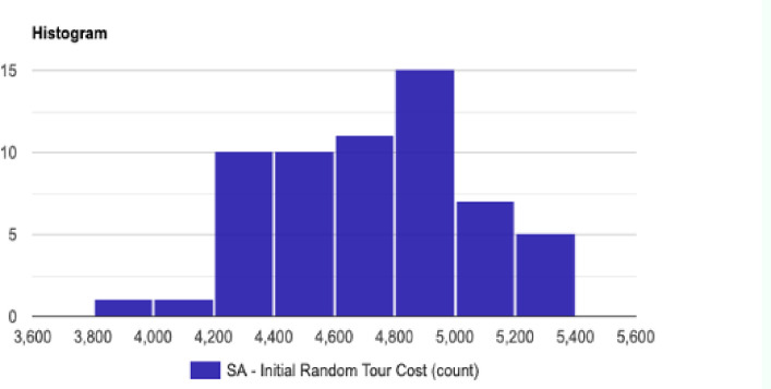
Histogram for the initial tour cost in the SA method.
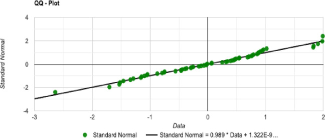
QQ-Plot for the initial tour cost in the SA method.
Shapiro-Wilk test, using a right-tailed normal distribution
H0 hypothesis
Since p-value > α, we accept the H0. It is assumed that the data is normally distributed. In other words, the difference between the data sample and the normal distribution is not big enough to be statistically significant.
P-value
p-value is 0.475660, hence, if we would reject H0, the chance of type1 error (rejecting a correct H0) would be too high: 0.4757 (47.57%). The larger the p-value, the more it supports H0
The statistics
W is 0.981075. It is in the 95% critical value accepted range: [0.9605: 1.0000]
Next we have created the boxplot graph to represent the median, average and the quartiles for QA and SA sample distributions.
Results from QA simulation: Best tour cost found
The statistical description for the QA method distribution with n = 50 nodes and length N = 60 is described as follow
Sample size: 60
Median: 897.3196982
Minimum: 700.0706523
Maximum: 1123.628464
First quartile: 829.287859975
Third quartile: 971.0301233
Interquartile Range: 141.742263325
Outliers: none
The boxplot for the QA distribution is illustrated in Fig 36
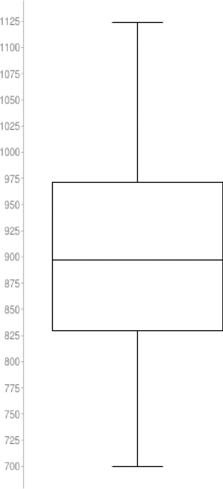
Boxplot for the QA simulation.
Results from SA simulation: Best tour cost found
The statistical description for the SA method distribution with n = 50 nodes and length N = 60 is described as follow
Sample size: 60
Median: 961.0134322
Minimum: 679.4900154
Maximum: 1358.45442
First quartile: 865.4905371
Third quartile: 1057.63755725
Interquartile Range: 192.14702015
Outlier: 1358.45442
The boxplot for the SA distribution is illustrated in Fig 37
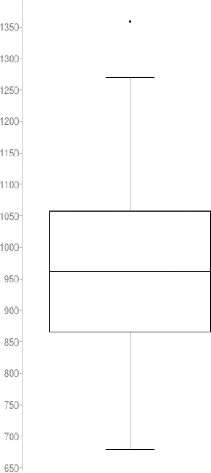
Boxplot for the SA simulation.
Test cases and computer simulation
The test cases are a set with 20, 30 and 50 nodes. The network latency between each node is bounded by the geographic distances between the machines, made available by the computing service provider. It’s the time required to send a message over a noisy communication channel. The proposed algorithm was used to find the optimal network route to deploy a process in a cluster of machines. In Tables 13–15 we present the Euclidian coordinates used to generate the candidate solutions and the cost matrix. We have provided a sample to demonstrate the results between QA and SA from the 180 trials (N = 60 for each sample). The data shows the first initial tour and the optimal solution found for each algorithm (the example data was extracted from the results produced by the simulations).
List of nodes with length N = 20 with coordinates (X, Y) in a 2D plan.
| Node | X | Y |
|---|---|---|
| 1 | 288 | 149 |
| 2 | 288 | 129 |
| 3 | 270 | 133 |
| 4 | 256 | 141 |
| 5 | 256 | 157 |
| 6 | 246 | 157 |
| 7 | 236 | 169 |
| 8 | 228 | 169 |
| 9 | 228 | 161 |
| 10 | 220 | 169 |
| 11 | 212 | 169 |
| 12 | 204 | 169 |
| 13 | 196 | 169 |
| 14 | 188 | 169 |
| 15 | 196 | 161 |
| 16 | 188 | 145 |
| 17 | 172 | 145 |
| 18 | 164 | 145 |
| 19 | 156 | 145 |
| 20 | 148 | 145 |
The QA simulation results are described with four variables
First solution path: ['1', '20', '8', '7', '17', '13', '2', '3', '16', '9', '15', '11', '14', '10', '6', '19', '4', '5', '18', '12']
Total distance cost from the first(starting) solution: 1145.7617186058662
Best solution Path: ['6', '5', '1', '2', '3', '4', '9', '15', '16', '17', '18', '19', '20', '14', '13', '12', '11', '10', '8', '7']
Total distance cost for the best solution found: 332.1144088148687
List of nodes with length N = 30 with coordinates (X, Y) in a 2D plan
| Node | X | Y |
|---|---|---|
| 1 | 288 | 149 |
| 2 | 288 | 129 |
| 3 | 270 | 133 |
| 4 | 256 | 141 |
| 5 | 256 | 157 |
| 6 | 246 | 157 |
| 7 | 236 | 169 |
| 8 | 228 | 169 |
| 9 | 228 | 161 |
| 10 | 220 | 169 |
| 11 | 212 | 169 |
| 12 | 204 | 169 |
| 13 | 196 | 169 |
| 14 | 188 | 169 |
| 15 | 196 | 161 |
| 16 | 188 | 145 |
| 17 | 172 | 145 |
| 18 | 164 | 145 |
| 19 | 156 | 145 |
| 20 | 148 | 145 |
| 21 | 140 | 145 |
| 22 | 148 | 169 |
| 23 | 164 | 169 |
| 24 | 172 | 169 |
| 25 | 156 | 169 |
| 26 | 140 | 169 |
| 27 | 132 | 169 |
| 28 | 124 | 169 |
| 29 | 116 | 161 |
| 30 | 104 | 153 |
The QA simulation results are described with four variables
First solution path: ['20', '24', '23', '9', '2', '6', '21', '15', '27', '1', '11', '14', '29', '25', '5', '28', '13', '7', '18', '22', '26', '4', '19', '12', '3', '17', '10', '30', '8', '16']
Total distance cost from the first(starting) solution: 2114.8616643887417
Best solution Path: ['4', '9', '12', '13', '14', '24', '23', '25', '22', '26', '27', '28', '29', '30', '21', '20', '19', '18', '17', '16', '15', '11', '10', '8', '7', '6', '5', '1', '2', '3']
Total distance cost for the best solution found: 423.26765018746386
List of nodes with length N = 50 with coordinates (X, Y) in a 2D plan
| Node | X | Y |
|---|---|---|
| 1 | 288 | 149 |
| 2 | 288 | 129 |
| 3 | 270 | 133 |
| 4 | 256 | 141 |
| 5 | 256 | 157 |
| 6 | 246 | 157 |
| 7 | 236 | 169 |
| 8 | 228 | 169 |
| 9 | 228 | 161 |
| 10 | 220 | 169 |
| 11 | 212 | 169 |
| 12 | 204 | 169 |
| 13 | 196 | 169 |
| 14 | 188 | 169 |
| 15 | 196 | 161 |
| 16 | 188 | 145 |
| 17 | 172 | 145 |
| 18 | 164 | 145 |
| 19 | 156 | 145 |
| 20 | 148 | 145 |
| 21 | 140 | 145 |
| 22 | 148 | 169 |
| 23 | 164 | 169 |
| 24 | 172 | 169 |
| 25 | 156 | 169 |
| 26 | 140 | 169 |
| 27 | 132 | 169 |
| 28 | 124 | 169 |
| 29 | 116 | 161 |
| 30 | 104 | 153 |
| 31 | 104 | 161 |
| 32 | 104 | 169 |
| 33 | 90 | 165 |
| 34 | 80 | 157 |
| 35 | 64 | 157 |
| 36 | 64 | 165 |
| 37 | 56 | 169 |
| 38 | 56 | 161 |
| 39 | 56 | 153 |
| 40 | 56 | 145 |
| 41 | 56 | 137 |
| 42 | 56 | 129 |
| 43 | 56 | 121 |
| 44 | 40 | 121 |
| 45 | 40 | 129 |
| 46 | 40 | 137 |
| 47 | 40 | 145 |
| 48 | 40 | 153 |
| 49 | 40 | 161 |
| 50 | 40 | 169 |
The QA simulation results are described with four variables
First solution path: ['38', '48', '39', '40', '9', '26', '28', '29', '33', '43', '41', '14', '12', '23', '1', '17', '20', '5', '49', '7', '35', '22', '18', '31', '6', '19', '13', '36', '2', '16', '42', '15', '4', '32', '25', '46', '8', '47', '50', '27', '37', '24', '34', '3', '10', '30', '45', '21', '44', '11']
Total distance cost from the first(starting) solution: 4919.680538441
Best solution Path: ['49', '48', '47', '41', '42', '43', '44', '45', '46', '40', '39', '38', '37', '36', '35', '34', '33', '32', '31', '30', '29', '21', '20', '19', '18', '17', '16', '9', '5', '1', '2', '3', '4', '6', '7', '8', '10', '11', '12', '15', '13', '14', '24', '23', '25', '22', '26', '27', '28', '50']
Total distance cost for the best solution found: 700.0706523445637
In Figs 38, 39 and 40 we have the line charts with the results for each test case. The figures demonstrate that the QA algorithms produces expected results with smaller cost and best quality in average than the benchmark SA method with smaller time requirements. In all cases the initial path loaded from the input files was randomly flushed before the algorithm execution to guarantee the results were not biased.
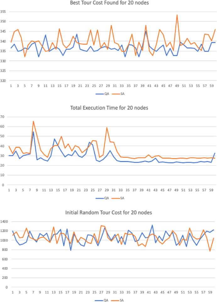
Chart with results for test cases with n = 20 nodes with sample size N = 60.
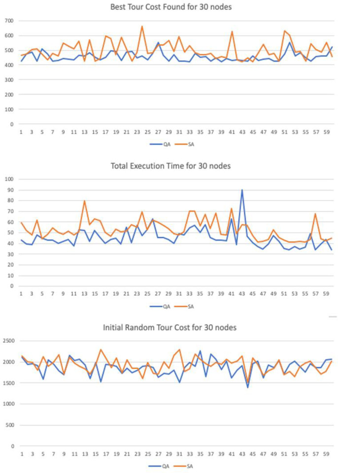
Chart with results for test cases with n = 30 nodes with sample size N = 60.
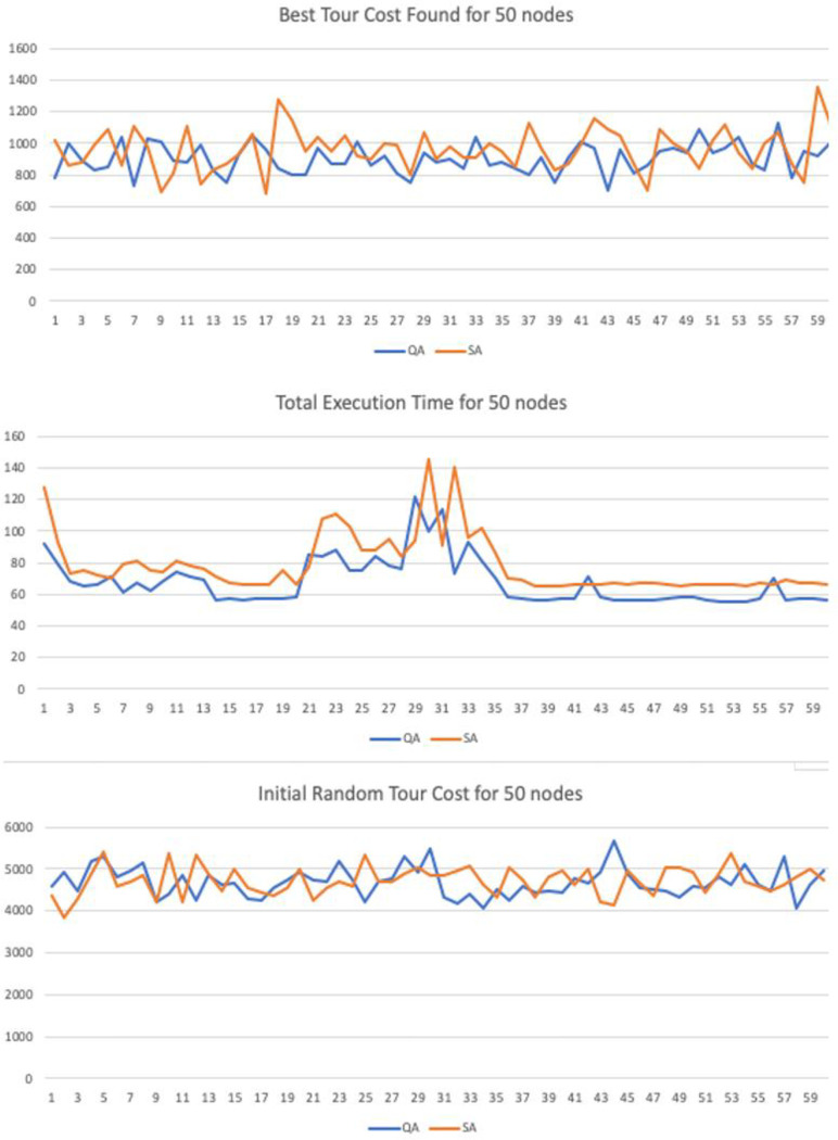
Chart with results for test cases with n = 50 nodes with sample size N = 60.
Tables 16–21 compares the results between the proposed algorithm and the heurists methods. They demonstrate that the result generated by the QA algorithm achieves solutions with better quality than the benchmark SA heuristic algorithm, by finding optimal solutions with smaller total cost and lesser running time. The QA algorithm converges more quickly than the 2opt algorithm for large instances of the problem. The results suggest the proposed Quantitative Algorithm is likely to perform better and generate consistent results as other traditional heuristics methods applied to the TSP. Additionally it provides an Information Theory modelling for Computationally Complex domains such as the NP class of problems in Turing Machines.
| t-Test: Two-Sample Assuming Unequal Variances | ||
|---|---|---|
| Cost Variable | ||
| QA | SA | |
| Mean | 336.552862 | 339.645729 |
| Variance | 6.35307736 | 18.1161823 |
| Observations | 60 | 60 |
| Hypothesized Mean Difference | 0 | |
| Df | 96 | |
| t Stat | -4.8431338 | |
| P(T< = t) one-tail | 2.4468E-06 | |
| t Critical one-tail | 1.66088144 | |
| P(T< = t) two-tail | 4.8935E-06 | |
| t Critical two-tail | 1.98498431 |
The result is significant at p < .05.
The 60 iterations who executed the QA algorithm (M = 336.552, Var = 6.353) compared to the 60 iterations in the SA algorithm (M = 339.645, Var = 18.116) demonstrated significantly better cost reduction, with value p = 4.8935E-06.
| t-Test: Two-Sample Assuming Unequal Variances | ||
|---|---|---|
| Execution Time Variable | ||
| QA | SA | |
| Mean | 28.1821012 | 34.06591929 |
| Variance | 43.5437993 | 69.06678708 |
| Observations | 60 | 60 |
| Hypothesized Mean Difference | 0 | |
| df | 112 | |
| t Stat | -4.2948228 | |
| P(T< = t) one-tail | 1.8689E-05 | |
| t Critical one-tail | 1.65857263 | |
| P(T< = t) two-tail | 3.7379E-05 | |
| t Critical two-tail | 1.98137181 |
The result is significant at p < .05.
The 60 iterations who executed the QA algorithm (M = 28.182, Var = 43.543) compared to the 60 iterations in the SA algorithm (M = 34.065, Var = 69.066) demonstrated significantly better time to complete execution, with value p = 3.7379E-05.
| t-Test: Two-Sample Assuming Unequal Variances | ||
|---|---|---|
| Cost Variable | ||
| QA | SA | |
| Mean | 455.9177842 | 500.1505 |
| Variance | 917.1905283 | 3396.48698 |
| Observations | 60 | 60 |
| Hypothesized Mean Difference | 0 | |
| df | 89 | |
| t Stat | -5.216694386 | |
| P(T< = t) one-tail | 5.88396E-07 | |
| t Critical one-tail | 1.662155326 | |
| P(T< = t) two-tail | 1.17679E-06 | |
| t Critical two-tail | 1.9869787 |
The result is significant at p < .05.
The 60 iterations who executed the QA algorithm (M = 455.917, Var = 917.190) compared to the 60 iterations in the SA algorithm (M = 500.150, Var = 3396.486) demonstrated significantly better cost reduction, with value p = 1.17679E-06.
| t-Test: Two-Sample Assuming Unequal Variances | ||
|---|---|---|
| Execution Time Variable | ||
| QA | SA | |
| Mean | 45.3019303 | 53.1616159 |
| Variance | 83.6019137 | 82.7521257 |
| Observations | 60 | 60 |
| Hypothesized Mean Difference | 0 | |
| df | 118 | |
| t Stat | -4.7202404 | |
| P(T< = t) one-tail | 3.2683E-06 | |
| t Critical one-tail | 1.65786952 | |
| P(T< = t) two-tail | 6.5365E-06 | |
| t Critical two-tail | 1.98027225 |
The result is significant at p < .05.
The 60 iterations who executed the QA algorithm (M = 45.301, Var = 83.601) compared to the 60 iterations in the SA algorithm (M = 53.161, Var = 82.752) demonstrated significantly better time to complete execution, with value p = 6.5365E-06.
| t-Test: Two-Sample Assuming Unequal Variances | ||
|---|---|---|
| Cost Variable | ||
| QA | SA | |
| Mean | 901.7845936 | 960.3116942 |
| Variance | 8917.028193 | 18189.17941 |
| Observations | 60 | 60 |
| Hypothesized Mean Difference | 0 | |
| df | 106 | |
| t Stat | -2.753583529 | |
| P(T< = t) one-tail | 0.003468798 | |
| t Critical one-tail | 1.659356034 | |
| P(T< = t) two-tail | 0.006937597 | |
| t Critical two-tail | 1.982597262 |
The result is significant at p < .05.
The 60 iterations who executed the QA algorithm (M = 901.784, Var = 8917.028) compared to the 60 iterations in the SA algorithm (M = 960.311, Var = 18189.179) demonstrated significantly better cost reduction, with value p = 0.006937597.
| t-Test: Two-Sample Assuming Unequal Variances | ||
|---|---|---|
| Execution Time Variable | ||
| QA | SA | |
| Mean | 67.6962824 | 78.4087974 |
| Variance | 215.812669 | 334.607097 |
| Observations | 60 | 60 |
| Hypothesized Mean Difference | 0 | |
| df | 113 | |
| t Stat | -3.5368778 | |
| P(T< = t) one-tail | 0.00029419 | |
| t Critical one-tail | 1.65845022 | |
| P(T< = t) two-tail | 0.00058839 | |
| t Critical two-tail | 1.98118036 |
The result is significant at p < .05.
The 60 iterations who executed the QA algorithm (M = 67.696, Var = 215.812) compared to the 60 iterations in the SA algorithm (M = 78.408, Var = 334.607) demonstrated significantly better time to complete execution, with value p = 0.00058839.
In the Appendix sections we have the Tables 22, 23 and 24 for the 3 test cases with nodes n = {20, 30, 50}, with the trial input variables for best final tour cost, total execution time and the initial tour cost for a sample length of N = 60. In Tables 19–21 we have the t-test p-value for each test case for the cost and execution time variable. Tables 16 and 17 demonstrate the T-test calculation for 2 independent means for n = 20.
| 20-node | ||||||
|---|---|---|---|---|---|---|
| Trial N = 60 | Initial Random Tour Cost | Best Tour Cost Found | Total Execution Time | |||
| 0 | QA | SA | QA | SA | QA | SA |
| 1 | 1195.634925 | 1108.393775 | 336.620892 | 339.439482 | 30.12948538 | 39.6077362 |
| 2 | 986.9352715 | 1177.732299 | 338.5615264 | 344.758321 | 30.26399596 | 32.3809037 |
| 3 | 900.0458995 | 1054.1641 | 334.8573413 | 345.966652 | 34.91276873 | 38.7632731 |
| 4 | 916.5463351 | 1057.927051 | 335.3011739 | 341.855037 | 27.23480984 | 38.4763941 |
| 5 | 966.1553232 | 1253.494224 | 336.620892 | 332.114409 | 29.91621914 | 32.1631082 |
| 6 | 1194.232179 | 1064.387485 | 335.8914965 | 338.044106 | 31.12498264 | 33.1915936 |
| 7 | 1036.191977 | 1029.253756 | 338.5615264 | 340.135251 | 31.81935215 | 32.060559 |
| 8 | 963.2410995 | 999.9887981 | 339.3638244 | 339.439482 | 54.49795967 | 65.4112282 |
| 9 | 1145.761719 | 1050.78347 | 332.1144088 | 340.059594 | 25.79352437 | 50.170809 |
| 10 | 1085.090655 | 1073.381069 | 337.2219503 | 337.316661 | 27.91745513 | 35.5128518 |
| 11 | 1147.417441 | 1012.068389 | 343.0294931 | 334.857341 | 25.94175636 | 31.4301689 |
| 12 | 965.8459042 | 958.2459652 | 334.8573413 | 335.301174 | 24.29773869 | 28.3900081 |
| 13 | 1128.489942 | 1283.781151 | 335.9022323 | 339.231552 | 29.54066219 | 37.4386245 |
| 14 | 1131.818667 | 928.6586146 | 337.0140207 | 335.902232 | 47.45874454 | 40.282868 |
| 15 | 1229.658241 | 1153.404679 | 335.9022323 | 346.41498 | 40.86180719 | 40.4422965 |
| 16 | 884.1357153 | 1138.13307 | 332.7154672 | 338.561526 | 34.48849958 | 49.9608527 |
| 17 | 1235.918025 | 1052.377384 | 335.9022323 | 336.620892 | 28.82108637 | 37.7635394 |
| 18 | 783.6900544 | 929.1934876 | 335.8914965 | 338.561526 | 31.23878077 | 42.0187519 |
| 19 | 1130.320419 | 1174.181378 | 337.0140207 | 342.439171 | 30.00009195 | 34.7658014 |
| 20 | 989.3865301 | 951.2563694 | 343.5134562 | 339.363824 | 35.36053606 | 40.5407622 |
| 21 | 904.2377617 | 1063.30281 | 335.9022323 | 338.741826 | 29.65111817 | 38.7390394 |
| 22 | 869.7243065 | 1029.595623 | 335.3011739 | 338.561526 | 28.38350387 | 32.86863 |
| 23 | 1116.176649 | 953.0821731 | 334.8573413 | 338.561526 | 31.87757207 | 36.2553472 |
| 24 | 1110.200886 | 931.6046509 | 337.3166611 | 345.685585 | 43.94790548 | 40.1406831 |
| 25 | 1064.184077 | 1139.258709 | 334.8573413 | 338.119763 | 41.20329418 | 45.7096829 |
| 26 | 887.1252702 | 940.9695223 | 335.3011739 | 345.685585 | 25.25219875 | 45.1240136 |
| 27 | 1040.447342 | 1308.425282 | 336.4925548 | 336.620892 | 23.90627663 | 28.4887706 |
| 28 | 1263.036989 | 1297.030551 | 337.2219503 | 339.231552 | 26.12993897 | 31.0484482 |
| 29 | 1115.022094 | 1055.582523 | 337.0140207 | 335.902232 | 29.95108272 | 58.9338429 |
| 30 | 998.9318306 | 981.3689839 | 335.9022323 | 348.044562 | 35.33063453 | 44.3207047 |
| 31 | 1127.712215 | 1066.313009 | 336.4129623 | 339.342884 | 28.56060964 | 43.9690071 |
| 32 | 945.3399049 | 1133.277072 | 335.3011739 | 338.561526 | 25.08187038 | 34.241621 |
| 33 | 1079.60359 | 913.4123438 | 338.0441064 | 334.857341 | 23.84379763 | 28.6076721 |
| 34 | 913.3758632 | 1151.462443 | 332.1144088 | 334.932998 | 24.00100185 | 28.4874175 |
| 35 | 1210.249512 | 1120.714135 | 338.3112039 | 338.561526 | 24.2204857 | 28.3244191 |
| 36 | 1147.723302 | 1130.778705 | 338.0441064 | 343.649497 | 23.43391117 | 27.3482798 |
| 37 | 971.3903556 | 1076.686391 | 336.620892 | 332.715467 | 23.04826988 | 27.2579731 |
| 38 | 998.2103312 | 887.1398159 | 332.1144088 | 339.439482 | 23.30005102 | 27.9801567 |
| 39 | 1162.280089 | 924.1853956 | 337.9177195 | 335.301174 | 23.55994665 | 28.0173068 |
| 40 | 1054.008142 | 869.5783019 | 345.095262 | 348.044562 | 24.4069206 | 28.0580326 |
| 41 | 1062.958346 | 1092.610068 | 337.3166611 | 334.857341 | 23.58406409 | 30.9849236 |
| 42 | 1316.550471 | 1132.915517 | 335.9022323 | 332.715467 | 24.49907442 | 27.7148466 |
| 43 | 944.5629418 | 1096.900034 | 334.8573413 | 338.561526 | 27.42394148 | 29.689707 |
| 44 | 1090.841136 | 973.9952212 | 336.620892 | 345.879822 | 23.22344759 | 30.1561858 |
| 45 | 985.9883167 | 915.8312807 | 338.0441064 | 343.428117 | 23.68698814 | 27.5134631 |
| 46 | 1193.337578 | 1001.967642 | 332.7154672 | 337.22195 | 23.15058773 | 27.6503922 |
| 47 | 1085.046538 | 1056.207841 | 336.4129623 | 339.439482 | 22.89809065 | 27.6979532 |
| 48 | 1170.592904 | 1204.896611 | 332.7154672 | 335.301174 | 22.811833 | 27.1470865 |
| 49 | 888.3716219 | 1119.310235 | 332.7154672 | 353.222205 | 23.53460078 | 27.1795784 |
| 50 | 957.744169 | 896.1779984 | 339.4394815 | 337.917719 | 22.97475352 | 27.4758247 |
| 51 | 1105.010107 | 1023.615603 | 338.0441064 | 338.710086 | 22.86918458 | 27.2797519 |
| 52 | 868.7296417 | 1001.961386 | 336.4925548 | 341.484758 | 23.09712953 | 27.1193013 |
| 53 | 1147.110698 | 1261.361139 | 336.620892 | 338.561526 | 23.20182619 | 27.8441451 |
| 54 | 1007.496906 | 1076.417337 | 336.4129623 | 339.231552 | 22.91703718 | 27.7154546 |
| 55 | 888.3254017 | 1028.532428 | 334.8573413 | 337.014021 | 23.08894057 | 27.652091 |
| 56 | 1015.389387 | 1037.982865 | 338.5615264 | 335.301174 | 24.19610564 | 27.4061656 |
| 57 | 1118.083211 | 1218.690552 | 334.8573413 | 343.500897 | 23.50864635 | 27.9921575 |
| 58 | 1196.871246 | 1056.936272 | 334.8573413 | 343.428117 | 23.84533973 | 27.6875045 |
| 59 | 1172.5209 | 765.331396 | 339.3638244 | 340.059594 | 23.19705539 | 27.9977026 |
| 60 | 1225.40291 | 1041.148332 | 339.3638244 | 345.962516 | 32.50677825 | 27.3577434 |
| 30-node | ||||||
|---|---|---|---|---|---|---|
| Trial N = 60 | Initial Random Tour Cost | Best Tour Cost Found | Total Execution Time | |||
| 0 | QA | SA | QA | SA | QA | SA |
| 1 | 2114.861664 | 2138.958342 | 424.5873682 | 464.700899 | 42.98706438 | 59.0712779 |
| 2 | 1941.575116 | 2007.049171 | 475.6796776 | 472.590934 | 39.46565883 | 52.120306 |
| 3 | 1950.142483 | 1989.063029 | 488.989852 | 504.453757 | 38.60825704 | 47.8920127 |
| 4 | 1902.474244 | 1796.927917 | 424.3794386 | 506.801158 | 48.13539106 | 61.4913984 |
| 5 | 1580.54924 | 2121.678062 | 510.318469 | 472.980497 | 44.92054756 | 44.2866884 |
| 6 | 2040.501524 | 1887.043741 | 474.6886065 | 433.933129 | 43.33821167 | 48.5092938 |
| 7 | 1933.189429 | 2005.284134 | 426.0105826 | 478.033092 | 43.31067901 | 54.8387858 |
| 8 | 1791.060214 | 2174.057473 | 429.9694289 | 462.536112 | 40.27118746 | 50.435126 |
| 9 | 1697.688572 | 1712.42956 | 443.4357473 | 548.033561 | 41.870426 | 48.4660826 |
| 10 | 2159.279821 | 2101.511052 | 439.9631361 | 526.162767 | 43.91304872 | 51.6482356 |
| 11 | 2037.032939 | 1964.471053 | 436.517103 | 507.74012 | 37.68801916 | 48.1148758 |
| 12 | 2057.901751 | 1892.015046 | 467.0236214 | 562.704654 | 52.46498072 | 51.1041011 |
| 13 | 1930.750408 | 1831.163179 | 460.014352 | 426.528003 | 52.34054281 | 79.7551805 |
| 14 | 1596.34284 | 1709.164989 | 484.0191023 | 571.764133 | 41.91429676 | 57.815061 |
| 15 | 1989.991866 | 1932.746628 | 453.6891305 | 428.101727 | 52.06071529 | 63.1093559 |
| 16 | 1532.819374 | 2294.07567 | 432.8197583 | 443.083125 | 45.44243764 | 61.380042 |
| 17 | 1933.611183 | 2091.996596 | 453.529067 | 595.347046 | 40.35533853 | 50.0510586 |
| 18 | 1928.551184 | 1860.347264 | 495.9653506 | 580.368162 | 43.90844072 | 46.7043453 |
| 19 | 1892.952203 | 2098.647235 | 491.0938606 | 468.450763 | 45.20533055 | 53.5513851 |
| 20 | 1727.389612 | 1746.213002 | 428.8730412 | 587.027872 | 39.56974309 | 50.744991 |
| 21 | 1840.460231 | 2052.640373 | 486.8539675 | 510.278944 | 55.44163731 | 51.324384 |
| 22 | 1734.505095 | 1843.716782 | 491.0156727 | 427.122371 | 40.87608984 | 57.7772876 |
| 23 | 1804.725607 | 1840.418372 | 447.2951117 | 486.01134 | 57.19451948 | 55.1076989 |
| 24 | 1900.969989 | 1597.14205 | 460.1507211 | 662.168972 | 47.51163171 | 69.8538226 |
| 25 | 1902.159287 | 1982.433073 | 433.0617383 | 477.980165 | 52.9507134 | 52.5828033 |
| 26 | 1861.379571 | 1732.215165 | 478.1275476 | 481.88559 | 63.18074776 | 61.506958 |
| 27 | 1632.125705 | 1705.527663 | 551.6573018 | 534.398358 | 45.71926259 | 59.901718 |
| 28 | 1724.804881 | 2004.34791 | 464.0476771 | 533.121258 | 45.68037277 | 57.0611448 |
| 29 | 1711.276107 | 1851.488894 | 426.6765623 | 565.016049 | 43.55173205 | 53.7347876 |
| 30 | 1798.24361 | 2147.552334 | 467.8403795 | 491.540871 | 39.89643796 | 48.881184 |
| 31 | 1505.540858 | 2286.236266 | 427.122371 | 592.196033 | 48.98996233 | 48.1386252 |
| 32 | 1868.889925 | 1772.226931 | 427.4357473 | 488.765595 | 47.68942928 | 50.6868412 |
| 33 | 1986.199157 | 1831.914237 | 423.8687085 | 530.861945 | 54.60683943 | 70.0300942 |
| 34 | 1893.774487 | 2191.409802 | 476.6245181 | 482.210099 | 56.77093291 | 69.9386231 |
| 35 | 2254.034678 | 2057.794281 | 450.6222049 | 470.823818 | 50.39574996 | 56.2931122 |
| 36 | 1641.972013 | 1951.754928 | 456.9229002 | 470.823818 | 57.52063273 | 67.2678736 |
| 37 | 2190.641527 | 1892.120281 | 427.1980282 | 479.691631 | 45.58968535 | 54.0853191 |
| 38 | 2059.180754 | 1991.897847 | 446.6225652 | 443.410875 | 43.33406437 | 68.1481031 |
| 39 | 1816.734006 | 1938.160932 | 423.2676502 | 457.649743 | 43.01746808 | 48.3186617 |
| 40 | 2009.362159 | 2057.941367 | 442.9039608 | 449.980838 | 42.63856604 | 48.0714487 |
| 41 | 1619.209653 | 1977.29523 | 430.5704872 | 625.975132 | 63.20465673 | 72.4023792 |
| 42 | 1803.072488 | 2008.969722 | 436.3291255 | 434.210099 | 38.81750628 | 49.0113726 |
| 43 | 1905.327122 | 2139.748939 | 431.6159736 | 422.823818 | 90.17018865 | 57.4507498 |
| 44 | 1396.063861 | 1510.800171 | 427.122371 | 446.937846 | 46.57496965 | 56.7508254 |
| 45 | 1961.970303 | 2085.66334 | 461.2238488 | 423.868709 | 40.88945298 | 47.0390539 |
| 46 | 2016.906558 | 1945.01613 | 431.6159736 | 482.392057 | 37.00943786 | 41.2652409 |
| 47 | 1615.747074 | 1679.767432 | 438.5243978 | 540.930956 | 34.94234454 | 41.9965412 |
| 48 | 1919.853209 | 1791.446699 | 442.7060685 | 468.628522 | 39.62350488 | 43.5543638 |
| 49 | 1864.485907 | 1841.077381 | 427.122371 | 478.851995 | 47.30976915 | 52.8924325 |
| 50 | 2033.030066 | 2044.268536 | 427.1980282 | 427.122371 | 41.87760103 | 45.4800351 |
| 51 | 1717.798426 | 1690.966193 | 474.7739314 | 629.184876 | 35.09427462 | 42.9087137 |
| 52 | 1943.528232 | 1778.978193 | 553.2831374 | 599.182846 | 34.25907436 | 41.3755334 |
| 53 | 2011.609188 | 1652.077927 | 460.8365081 | 489.159339 | 36.82620546 | 41.3364099 |
| 54 | 1893.324832 | 1873.394732 | 483.4554998 | 491.107552 | 34.69045473 | 41.6829564 |
| 55 | 1761.65708 | 1971.263332 | 448.7644393 | 426.010583 | 36.35978929 | 41.3863896 |
| 56 | 1948.645928 | 2020.716704 | 428.0260698 | 542.400253 | 48.97381794 | 43.9572916 |
| 57 | 1867.947796 | 1850.588061 | 455.8265125 | 505.167828 | 34.33525243 | 67.9172457 |
| 58 | 1858.698459 | 1717.237261 | 461.1244452 | 485.823316 | 39.20625309 | 44.2034129 |
| 59 | 2046.855774 | 1778.212757 | 461.5046079 | 554.4155 | 43.44987886 | 42.5260492 |
| 60 | 2054.476294 | 2022.162447 | 522.5612263 | 457.556595 | 34.17459443 | 44.7598619 |
| 50-node | ||||||
|---|---|---|---|---|---|---|
| Trial N = 60 | Initial Random Tour Cost | Best Tour Cost Found | Total Execution Time | |||
| 0 | QA | SA | QA | SA | QA | SA |
| 1 | 4584.994704 | 4350.530615 | 783.6135781 | 1013.45381 | 91.94147284 | 127.121441 |
| 2 | 4931.04388 | 3829.72755 | 1002.266343 | 856.714194 | 79.49352819 | 93.1328427 |
| 3 | 4459.545641 | 4285.493079 | 892.4679561 | 878.335327 | 67.90769484 | 73.4395111 |
| 4 | 5189.508014 | 4873.122362 | 825.1186081 | 986.814761 | 65.57152077 | 74.8066559 |
| 5 | 5303.265261 | 5389.224823 | 846.448402 | 1085.77975 | 65.92321619 | 72.4844698 |
| 6 | 4792.633045 | 4595.016823 | 1036.163983 | 855.195737 | 71.40535116 | 70.3046693 |
| 7 | 4951.587728 | 4711.457297 | 735.82339 | 1110.36984 | 61.43196151 | 78.8009844 |
| 8 | 5127.650419 | 4851.865628 | 1028.714485 | 974.535522 | 67.16026587 | 80.7510912 |
| 9 | 4213.123791 | 4227.131367 | 1006.163651 | 693.015657 | 61.80173641 | 75.0614487 |
| 10 | 4388.805181 | 5361.415343 | 887.0345646 | 813.130685 | 68.36587932 | 73.5915055 |
| 11 | 4862.966377 | 4203.513913 | 877.8178844 | 1104.47353 | 73.62834893 | 81.1984111 |
| 12 | 4265.85426 | 5334.298362 | 986.2523487 | 742.17075 | 70.93162192 | 78.2357104 |
| 13 | 4830.792434 | 4901.318711 | 826.6711289 | 827.602189 | 68.93372081 | 76.0991019 |
| 14 | 4619.684576 | 4464.911989 | 749.4744233 | 871.360054 | 56.4622385 | 71.1095197 |
| 15 | 4672.945496 | 5012.768994 | 930.1932444 | 930.647017 | 57.45928662 | 66.9842984 |
| 16 | 4301.693121 | 4563.371791 | 1048.809952 | 1059.51057 | 56.40269137 | 66.0322041 |
| 17 | 4240.292119 | 4453.55102 | 960.9380585 | 679.490015 | 57.05427107 | 66.3409535 |
| 18 | 4546.900924 | 4368.046961 | 837.1380532 | 1269.71181 | 57.57915765 | 66.263964 |
| 19 | 4736.784109 | 4563.713271 | 803.5690309 | 1149.69257 | 57.39472165 | 75.1020043 |
| 20 | 4927.370618 | 4985.626756 | 802.0707333 | 949.201069 | 58.56337916 | 66.5018131 |
| 21 | 4745.962526 | 4268.210716 | 971.2161657 | 1035.84231 | 84.97886224 | 77.278123 |
| 22 | 4704.060283 | 4530.930051 | 871.0047479 | 946.415563 | 83.75003637 | 107.235943 |
| 23 | 5181.527463 | 4709.96614 | 869.6858203 | 1049.75812 | 88.00241065 | 110.964508 |
| 24 | 4718.091802 | 4570.219583 | 1003.026828 | 917.555919 | 74.77390515 | 102.335962 |
| 25 | 4226.097192 | 5336.282205 | 863.4354307 | 897.940395 | 74.88039926 | 88.0454088 |
| 26 | 4706.978399 | 4680.602383 | 919.2626516 | 999.01329 | 84.28058593 | 87.6437221 |
| 27 | 4782.240302 | 4696.840091 | 805.5766865 | 988.048877 | 77.9414429 | 94.365899 |
| 28 | 5287.422498 | 4883.631664 | 746.8961081 | 797.72096 | 76.3188141 | 84.3477808 |
| 29 | 4916.756496 | 5036.485112 | 934.4805999 | 1063.60839 | 121.2328974 | 94.1907275 |
| 30 | 5467.182912 | 4862.394357 | 881.0823054 | 898.962836 | 99.58652921 | 145.672337 |
| 31 | 4306.529303 | 4833.371655 | 902.1714403 | 982.659335 | 113.7672365 | 90.4546303 |
| 32 | 4183.027842 | 4974.432819 | 838.7087408 | 909.242445 | 72.86395342 | 140.711226 |
| 33 | 4392.939578 | 5062.464887 | 1037.318628 | 912.246168 | 93.25543078 | 96.0741311 |
| 34 | 4047.530913 | 4624.516897 | 855.2813664 | 997.411612 | 80.5475141 | 101.864948 |
| 35 | 4529.583132 | 4333.230947 | 877.4782972 | 948.148568 | 70.2493321 | 85.4985131 |
| 36 | 4255.799236 | 5016.586688 | 844.0019669 | 851.668489 | 58.39587275 | 69.6642768 |
| 37 | 4591.115727 | 4742.024106 | 801.0967517 | 1122.03704 | 57.4895984 | 68.7700118 |
| 38 | 4446.710076 | 4328.66242 | 908.2987592 | 972.825796 | 56.3946521 | 65.6056279 |
| 39 | 4463.651251 | 4803.549729 | 750.8183686 | 831.071231 | 55.89729563 | 65.1255863 |
| 40 | 4420.655007 | 4951.243552 | 909.1278545 | 866.473154 | 57.14852512 | 65.213147 |
| 41 | 4760.124614 | 4634.478576 | 1011.834532 | 987.252055 | 57.32113831 | 66.0356184 |
| 42 | 4644.224719 | 4979.032088 | 964.2360348 | 1157.92977 | 71.29050156 | 66.2798815 |
| 43 | 4919.680538 | 4208.101093 | 700.0706523 | 1085.31132 | 57.79070051 | 66.251104 |
| 44 | 5651.239742 | 4145.447347 | 955.4124378 | 1052.01851 | 56.53862412 | 66.9480465 |
| 45 | 4868.697543 | 4959.720826 | 813.4887026 | 872.689612 | 56.64083376 | 66.3630462 |
| 46 | 4548.266669 | 4667.805502 | 857.9641925 | 698.448853 | 56.46022322 | 67.1403534 |
| 47 | 4526.748229 | 4364.07524 | 944.2137708 | 1083.92177 | 56.08612165 | 67.1104689 |
| 48 | 4477.883901 | 5024.492103 | 972.2009554 | 999.856492 | 57.63071399 | 66.3520515 |
| 49 | 4317.125097 | 5044.001873 | 933.6392304 | 948.603177 | 58.23602575 | 65.5457691 |
| 50 | 4575.872243 | 4903.155907 | 1087.920943 | 839.863471 | 57.96136195 | 66.182039 |
| 51 | 4563.047938 | 4424.909203 | 934.2368709 | 1019.90042 | 56.72733254 | 65.8799768 |
| 52 | 4820.853628 | 4875.868205 | 970.4719961 | 1112.21415 | 55.71390442 | 66.183776 |
| 53 | 4615.052748 | 5386.727246 | 1034.389805 | 939.401344 | 55.77318577 | 65.8460782 |
| 54 | 5105.564284 | 4715.986396 | 873.7197202 | 836.813936 | 55.55562469 | 65.2542301 |
| 55 | 4633.267827 | 4585.63924 | 825.4093226 | 996.826956 | 57.06582138 | 66.729305 |
| 56 | 4487.584383 | 4467.312127 | 1123.628464 | 1071.80932 | 70.06335915 | 66.4194826 |
| 57 | 5282.957016 | 4620.83047 | 779.0921158 | 865.162998 | 56.55935544 | 69.5257076 |
| 58 | 4045.585905 | 4825.07628 | 944.2176677 | 747.969855 | 56.93291826 | 67.0270058 |
| 59 | 4633.980055 | 5006.414463 | 918.037855 | 1358.45442 | 57.70211316 | 66.7727485 |
| 60 | 4957.692367 | 4740.435311 | 1006.171011 | 1104.39786 | 56.55972443 | 66.2560434 |
These findings can be expanded to other complex problems and it scales linearly to the search space sample. The proposed method is also resistant to the time and space constraints and it has a constant number of maximum iterations. In this paper we have introduced a new interpretation for the entropy rate for a binary program that implements a given NP problem.
The results can be used by many real-world applications such as the optimization of routing messages over a network and the orchestration of services across a distributed system such as provided by Cloud Computing environments and micro-services-oriented architectures. Besides it is also a future reference on the subject of Information Theory, Computational Complex Theory and Logarithmic utility in optimization routing, deployment, scheduling and planning. The research demonstrated that the proposed concepts have statistically significant results with better solution quality in tour planning. The model provides a new interpretation of entropy in problems encoded in Turing Machines and has the potential to change the traditional interpretation of the limits of Computing Theory.
The results are statistically significant (with p-value < 0.05), and we can conclude the proposed algorithm has better solution quality with reduced computational requirements and better cost improvement.
Statistical analysis of the test cases
In order to test the performance in solving the TSP we have created trials with sample length N = 60 for each test case with different number of nodes n = {10, 30, 50} and then compared the results obtained with a benchmark heuristic (SA) and the proposed algorithm (QA).
Table 25 demonstrate the two-tailed t-test for two independent samples of costs and times measurements with Significance Level of 0.05. This is a two-sided test for the null hypothesis with two independent means have the identical expected value. This test measures if the average expected cost and running time value differs significantly across the measured samples. If the p-value is small than the significance level of 0.05 (5%) then we can reject the null hypothesis of equal average means.
| 20-node | 30-node | 50-node | |
| Cost variable t-test for N = 60 | QA-SA. | QA-SA. | QA-SA. |
| p-value | 4.89351E-06 | 1.17679E-06 | 0.0069376 |
| 20-node | 30-node | 50-node | |
| Time variable t-test for N = 60 | QA-SA. | QA-SA. | QA-SA. |
| p-value | 3.73787E-05 | 6.53652E-06 | 0.00058839 |
The Table 25 shows that results are statistically significant (with p-value < 0.05) for test cases n = {20, 30, 50}, and we can conclude the proposed Quantitative Algorithm (QA) has better solution quality with reduced computational requirements and better cost improvement than benchmark heuristic Simulated Annealing (SA).
Simulation review
As with any heuristics and metaheuristics, it is not an exact process defined by a general linear function, but the results from the statistical analysis demonstrate the algorithm’s quality are significant. In this paper we have demonstrated the statistical significance of the results, as the p-value for the t-Test with Unequal Variances between the Simulated Annealing (SA) heuristic (Benchmark) and the proposed Quantitative Algorithm (QA), is less than the significance level for alpha with p< 0.05. The statistical test was performed for graphs with 20, 30 and 50 nodes and all trials have returned a significant result by rejecting the null hypothesis.
This supports the evidence that the schema proposed by heuristics methods such as GA, SA, AC or CE produces results that are, in average, equal or worse than the proposed QA method based in Information Theory and Entropy simulation, running for the same number of finite iterations. The best cost and running time are in average, found in the sample from the QA method, although it was also found in the control group SA, used as our benchmark. This result is expected, as outliers can happen and are expected to be found in random process in the long term.
The results obtain in this research showed a smaller runtime overhead in QA method possibly because of the simpler numerical calculations and instructions set in the code, if compared to the above-mentioned traditional heuristics. In GA, SA, AC and Neural Networks for example there are complex matrix, string and graph manipulations.
The Christofides algorithm also has to keep track and detect short-cuts between nodes in the know state search-space and thus increasing memory requirements. The proposed method does not need a buffer of illegal moves, such as proposed by the Tabu search method used to optimize the k-opt algorithm.
It also doesn’t need to continuously look for short-cuts or swapping ties, it works by generating a random sequence that encode a Hamiltonian graph (i.e. A path that visits all nodes exactly once). After generating the random candidate solution there are only 3 conditions to decide:
Have we reached the maximum number of iterations defined in the input parameters? If yes than halt
If new path is better than the current best route than updates the current control state.
If the candidate solution is worse, than we accept the solution, according to a decaying Bernoulli process B(X) for random variable X and a probability density function estimation with entropy H(X) with dependent utility function Y = g(X).
Applications for the method
The Traveling Salesman Problem is the foundation for many optimization methods, algorithms, models and process with applications in many areas and fields such as
Computer science
◦ Optimize package routing for sending and receiving messages in a network ◦ Task Scheduling for batch processing in a cluster of servers
Logistics
◦ Optimize package and mail delivery between addresses in a city ◦ Vehicle route optimization for GPS systems ◦ Job shop problem to assign activities to a pool of resources ◦ Minimize the total execution length schedule of a set of tasks (makespan)
Fig 41 illustrates some applications of the TSP for shortest driving route, maximize server utilization and minimize makespan.
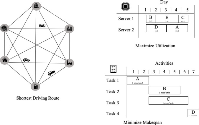
Example of TSP applications.
Conclusion
Service scheduling and network routing has many applications and is related to the optimization problem modeled by the Traveling Salesman Problem. It’s possible to improve performance by reducing the cost of transmission of information across many distributed systems locations. A new interpretation and verified optimization algorithm and statistical model based in Information Theory is presented in this paper and it demonstrated how it can be used to solve the TSP. The results support the idea that the proposed method can be used reliably to generate solution under a given degree of freedom. The algorithm can be expanded to large scale problems without the high requirements of computational resources utilization imposed by the brute-force and traditional heuristics methods such as Simulated Annealing, Ant Colony, Neural Networks and Genetic Algorithms. The algorithm can be adapted to any case of the routing problem. The research can be used as a framework for future works and extend the implications of Information Theory and Kolmogorov-Complexity in solving TSP and NP Problems in general.
The advantage of this approach is that it is independent of the computer encoding the problem and the time and space complexities are additive up to a limit that is linearly proportional to the input size. Other heuristics methods assume a predefined knowledge about the data structure and thus are biased towards this encoded schema. The implications of this interpretation is that by reducing the NP problems to a matter of modularization of encoded and decoded random signals in an communication noisy channel, we can find near optimal solutions that are statistically significant and are guaranteed to produce the best rate of improvement in the long run over many trials(i.e. simulation iterations) even though the problems itself is computationally complex and the alternative sequential brute force algorithm would require exponential time to solve. This mathematical model can be interpreted as a generalization of heuristics methods.
The findings in this paper unifies critical areas in Computer Science, Mathematics and Statistics that many researchers have not explored and provided a new interpretation that advances the understanding of the role of entropy in decision problems encoded in Turing Machines.
References
1
2
3
4
5
6
7
8
9
10
11
12
13
14
15
16
17
18
19
20
21
22
23
24
25
26
27