Rotamer library approach

Rotamer libraries have a long history in protein structural analysis [31], with an early application being to study side-chain packing [32]. Several other applications of this approach were later employed, e.g. in homology modeling and protein design [33, 34]. In our implementation, the RLA is used to insert the rotamer conformations of a paramagnetic probe at the spin-labeled site and to calculate the Boltzmann weight of each conformer. By default, we use the MTSSL 175 K rotamer library by Polyhach et al. [24], which was filtered to include only the χ₁ χ₂ conformations that are most commonly found in crystal structures of T4 Lysozyme [35]. As shown by Klose et al. [26], this selection criterion increases the accuracy of the calculated electron-electron distance distributions. The code is, however, general and it is possible to add new rotamer libraries by providing a text file containing the Boltzmann weights of each rotamer state $$ p_i^{int}$$, a topology file (PDB format) and a trajectory file (DCD format) where rotamers are aligned with respect to the the plane defined by Cα atom and C–N peptide bond. These files should be included in the lib folder and listed in the yaml file DEERPREdict/lib/libraries.yml. The default MTSSL 298 K MC/UFF CαSδ rotamer libraries of the Matlab-based MMM modeling toolbox [13] are also provided in the DEER-PREdict package.

Following the alignment of the rotamer to the protein backbone (Cα, C and N atoms), the calculation of the Boltzmann weights is based on the sum of internal, $$ {ϵ}_i^{int}$$, and external, $$ {ϵ}_i^{ext}$$, energy contributions. The internal contribution is taken from Polyhach et al. [24] and results from the clustering of representative dihedral combinations from MD simulations. The normalized frequency of each cluster throughout the MD trajectory was used to determine the Boltzmann probability, $$ p_i^{int}$$, of a given i^th state, which readily can be converted into an internal energy contribution, $$ {ϵ}_i^{int}$$, via Boltzmann inversion. On the other hand, the external energy contribution is calculated on the fly as the dispersion interaction energy between heavy atoms of rotamer and protein residues within a 1-nm cutoff, using the pairwise 6-12 Lennard-Jones potential of the CHARMM36 force field, with atom sizes scaled by the input parameter sigma_scaling, which defaults to 0.5 as in the MMM modeling toolbox (http://www.epr.ethz.ch/software) [13].

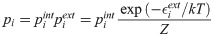
The overall probability of the i^th rotamer state is then calculated as

Predicting the DEER signal from structural ensembles

Electron-electron distance distributions extracted from DEER experiments, e.g. using the DeerLab package [36], have previously routinely been compared with distributions predicted using the RLA implemented in the Matlab-based MMM modeling toolbox (http://www.epr.ethz.ch/software) [13]. Since MMM intrinsically operates on single structures, we and others had to resort to wrapper scripts to compute distance distributions of large ensembles, such as MD trajectories [3, 25, 37]. With the program presented herein, we provide a tool to conveniently predict DEER distance distributions from large conformational ensembles, which can be easily integrated in reweighting schemes such as the Bayesian/maximum entropy procedure [1, 14, 38, 39].

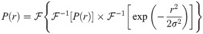
For each trajectory frame or conformation of a given ensemble, the rotamers from the library are placed at the spin-labeled position (Fig 1A) and the distances between all pair combinations of N-O paramagnetic centers are calculated. The resulting matrix of pair-wise distances is then used to compute the distance distribution weighted by the combined probability of each probe conformation, p_i × p_j, with p_i and p_j being the conformation probabilities of rotamers i and j. After averaging over all the frames, a low-pass filter is applied to the distance distribution for noise reduction [40],

Fig 1

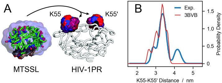
Probe placement scheme and comparison to DEER data.

(A) A pool of 46 conformations of the MTSSL probe from the rotamer library are aligned to the backbone of residues K55 and K55’ of HIV-1 protease. The color code represent the Boltzmann weights of each rotamer, increasing from blue to red. (B) Electron-electron distance distribution for HIV-1 protease spin labeled at residues K55 and K55’. The blue line is the experimental data from Torbeev et al. [44] whereas the red line is the prediction using DEER-PREdict and a crystal structure of HIV-1 protease (PDB code 3BVB).

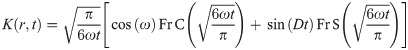
The dipolar modulation signal can be back-calculated from the distance distribution, P(r), via the following integral [41]

Prediction of PRE rates and intensity ratios

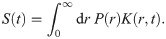
In analogy to the calculations of electron-electron distances to predict DEER distributions, we extended the use of the RLA to electron-proton separations to improve the accuracy of PRE predictions. We focus here is on PRE NMR experiments that probe the increase in transverse relaxation rates of any backbone proton due to the dipolar interaction with the unpaired electron of the paramagnetic probe:

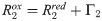
A description of the enhancement of the transverse relaxation due to dipole-dipole interactions in paramagnetic solutions was first proposed by Solomon and Bloembergen [45, 46]

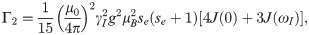
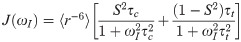
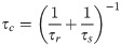
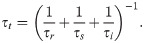
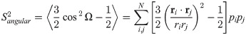
For the generalized order parameter, S, we use the factorization into contributions from radial and angular internal motions introduced by Brüschweiler et al. [49], $$ S^2=S_{radial}^2{S}_{angular}^2$$. The expressions for $$ S_{radial}^2$$ and $$ S_{angular}^2$$ were derived from a jump model that treats the N conformers of the rotamer library as N discrete states with equal probabilities (1/N) [50]. In reality, the various dihedral angles of the spin label have different free energy barriers, resulting in residence times between jumps ranging from less than 1 to several ns [17].

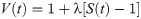
For samples with particularly high PRE rates it can be infeasible to obtain Γ₂ from multiple time-point measurements [60]. In such and other cases, the PRE is sometimes probed indirectly from the ratio of the peak intensities in ¹H,¹⁵N-HSQC spectra of the spin-labeled protein in the oxidized and reduced state. Assuming that the intensity of the proton magnetization decays exponentially—by transverse relaxation only—during the total INEPT time of the HSQC measurement [61], t_d, the intensity ratio is estimated as

Requirements and installation

The main requirements are Python 3.6–3.8 and MDAnalysis 1.0 [30, 62]. In an environment with Python 3.6–3.8, DEER-PREdict can readily be installed through the package manager PIP by executing

1 pip install DEERPREdict

Package stability

Tests reproducing DEER and PRE data for the protein systems studied in this article, as well as for a nanodisc [29], are performed automatically using Travis CI (travis-ci.com/github/KULL-Centre/DEERpredict) every time the code is modified on the GitHub repository. The same tests can also be run locally using the test running tool pytest.

Case study 1: DEER data for HIV-1 protease

HIV-1 protease (HIV-1PR) is a homodimeric aspartic hydrolase involved in the cleavage of the gag-pol polyprotein complex. The inhibition of this process affects the life cycle of the HIV-1 virus, rendering it noninfectious [63]. The HIV-1PR monomer is composed of 99 residues and presents a structurally stable core region (residues 1-43 and 58-99) and a dynamic region characterized by a β-hairpin turn, called the flap (residues 44-57). The active site is located at the interstice between the core regions of the two monomers, in proximity to the catalytic D25 residues. This cavity is closed off by the dynamic flap regions, which are considered to act as a gate controlling the access to the active site. The dynamics of the flap regions are of utmost importance for the development of inhibitors, and have been extensively studied, both experimentally and in silico [44, 64–69]. Based on the relative position of the flaps, three main conformational states have been proposed. In X-ray crystallography, the closed state is typically observed for the ligand-bound enzyme (e.g. PDB codes 3BVB [70] and 2BPX [71]), the semi-open state is predominant for the apo form (e.g. PDB code 1HHP [72]) whereas the wide-open state has been observed for variants (e.g. PDB codes 1TW7 [73] and 1RPI [74]) [69]. In DEER measurements, these conformational states can be resolved by spin-labeling sites K55 and K55’ (see S1 Text and S2 Fig).

To assess the predictive ability of DEER-PREdict, we generated conformational ensembles of the HIV-1PR homodimer via two different approaches: (a) a single 500-ns unbiased MD simulation, and (b) four independent 125-ns MD simulations restrained with experimental residual dipolar couplings (RDC) data [58, 75] from Roche et al. [65, 66] (see S1 Text for methodological details). The initial configuration of our simulations is the X-ray crystal structure of the active-site mutant D25N bound to the inhibitor Darunavir (PDB code 3BVB).

Fig 2 presents a comparison of experimental DEER distance distributions and echo intensity curves with predictions from simulation trajectories of 1,000 frames sampled every 0.5 ns. The echo intensity curves are calculated using Eq 6, where the λ is estimated to 0.0922 by fitting the experimental dipolar evolution function to the corresponding curve derived from the experimental P(r) via Eq 3. For a single trajectory, the analysis is performed in 13 s on a 1.7 GHz processor by running the following code:

1 import MDAnalysis

2 from DEERPREdict.DEER import DEERpredict

3 u = MDAnalysis.Universe(’conf.pdb’,’traj.xtc’)

4 DEER = DEERpredict(u,residues =[55, 55],chains=[’A’,’B’],temperature = 298)

5 DEER.run()

The third line generates the MDAnalysis Universe object from an XTC trajectory and a PDB topology. The fourth line initializes the DEERpredict object with the spin-labeled residue numbers and the respective chain IDs. The fifth line runs the calculations and saves per-frame and ensemble-averaged data to res-55-55.hdf5 and res-55-55.dat, respectively, as well as the steric partition functions of sites K55 and K55’ to the file res-Z-55-55.dat.

Fig 2

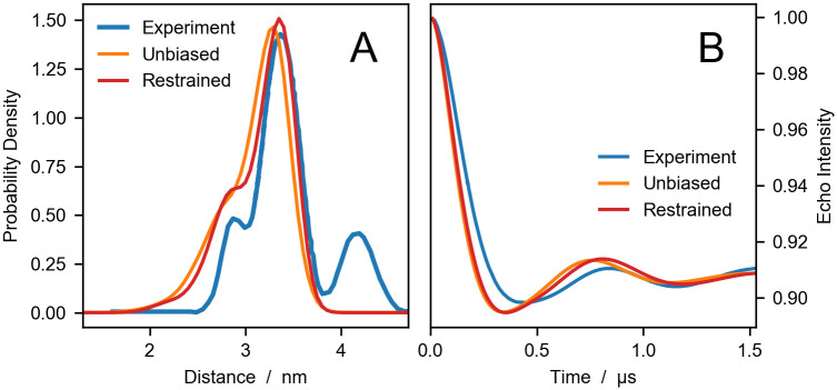
Comparing experiments and simulations for HIV1-PR.

DEER distance distributions (A) and echo intensity curves (B) obtained by Torbeev et al. [44] from DEER experiments (blue), and calculated using DEER-PREdict from unbiased (orange) and RDC ensemble-biased MD simulations (red).

In the experimental distance distribution, the main peak at ∼3.3 nm corresponds to the closed state whereas the second peak between 4 and 5 nm is characteristic of the wide-open state. The shoulder peak at ∼2.8 nm has been identified as an open-like state known as the curled/tucked conformation [9, 76, 77]. The results of our unbiased and restrained simulations are in substantial agreement with the findings of Roche et al. [65, 66], indicating that the flaps of the inhibitor-free HIV-1PR are predominantly in closed conformation. Compared to the distance distribution calculated from the starting configuration of PDB code 3BVB (see Fig 1), predictions based on MD trajectories more accurately reproduce the shape of the shoulder and the main peak of the experimental P(r). Moreover, using the RDC data as restraints leads to a significant improvement in the agreement between simulations and experiments, with the RMSD decreasing from 0.07 for the unbiased to 0.03 for the RDC ensemble-biased simulations. However, in the simulations we do not observe the wide-open state. This discrepancy could be due to insufficient sampling or could be attributed to the difference in sequence between the simulated protein and the experimental construct.

Case study 2: DEER data for T4 lysozyme

Lysozyme from the T4 bacteriophage (T4L) has long been used as a model system in the study of protein structure and dynamics [78–83]. Here, we focus on the L99A and the triple L99A-G113A-R119P mutants which are structurally similar and mainly differ in the relative populations of their major conformational states. The L99A variant presents a 150 ų hydrophobic pocket capable of binding hydrophobic ligands and has been thoroughly studied to further our understanding of the dynamics and selectivity of the binding pocket [78, 84]. The L99A variant occupies two distinct conformational states: the ground state (G) and the transient excited state (E), amounting for 97% and 3% of the population, respectively. The large-scale motions converting the G into the E state occur on the millisecond time scale and result in the occlusion of the cavity, which is occupied by the side chain of F114 in the E state [82]. The additional G113A and R119P mutations in the triple-mutant variant interconvert the populations of the conformational states to 4% for the G state and 96% for the E state [82]—note that, here and in the following, we refer to the G and E states based on their structural similarity to the L99A variant rather than on their relative populations. These conformational equilibria have been studied by DEER for various pairs of spin-labeled sites, which effectively resolve the G and E states as separate peaks of the P(r) [83].

Here, we compare DEER distance distributions calculated with DEER-PREdict for two pairs of probe positions (D89C–T109C and T109C–N140C) with the corresponding experimental data by Lerch et al. [83]. First, we calculate the P(r) of the single states using PDB code 3DMV for the G states and PDB codes 2LCB and 2LC9 for the E states of single and triple mutants, respectively. Second, the P(r)’s are linearly combined based on the experimentally derived ratios of G and E populations (97:3 for L99A and 4:96 for L99A-G113A-R119P) [82]. Additionally, we predict DEER distance distributions from previously reported metadynamics MD simulations of L99A and L99A-G113A-R119P [80] (see S1 Text for methodological details). In these calculations, the average over the trajectory is weighted by exp(F_bias/k_BT), where F_bias is the final static bias for each frame and k_BT is the thermal energy. The analysis of a trajectory of 6,670 frames is performed in 3 min on a 1.7 GHz processor executing the following lines of code:

1 import MDAnalysis

2 from DEERPREdict.DEER import DEERpredict

3 import numpy as np

4 u = MDAnalysis.Universe(’conf.pdb’,’traj.xtc’)

5 for residues in [[89, 109],[109, 140]]:

6  DEER = DEERpredict(u,residues = residues,temperature = 298,z_cutoff = 0.1)

7  DEER.run(weights = np.exp(Fbias/(0.298*8.3145)))

In line six, we specify the positions of the spin-labels, the temperature at which the metadynamics simulations were performed and a non-default value for the Z cutoff. In line seven, we provide the weights of each trajectory frame, generated from the array of F_bias values.

Fig 3 shows a comparison between the experimental distance distributions obtained by Lerch et al. [83] and our predictions. In general, the calculated distributions fall within the experimental ranges of inter-probe distances and are particularly accurate for the D89C–T109C spin-labeled pair in metadynamics simulations. The sharper shape of the experimental P(r)’s, relative to the calculated distributions, could be due to the cryogenic temperatures at which DEER experiments are conducted, whereas simulations were performed at room temperature. For the T109C–N140C spin-labeled pair of the triple variant, the discrepancy between predicted and calculated P(r)’s might be explained by considering that distances shorter than 1.5 nm fall below the range probed by DEER experiments. On the other hand, the inaccurate predictions of the T109C–N140C P(r) for the single (L99A) variant is greater than expected. Such discrepancies may be due both to errors in the protein structure or in the DEER-calculations. While our results cannot distinguish between these scenarios, we follow previous work [14] by examining whether the discrepancies can can be attributed to the error on the Boltzmann probabilities of the rotamer states, $$ p_i^{int}$$. We thus use a Bayesian/maximum entropy (BME) procedure to show that a small change in the original rotamer weights can lead to a substantial improvement of the agreement with the experimental data (see S1 Text and S3 Fig).

Fig 3

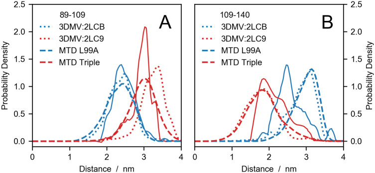
Comparing experiments with simulations and structures of T4 lysozyme variants.

DEER distance distributions for probe positions (A) D89C–T109C and (B) T109C–N140C of the single (blue) and the triple variant (red). Solid lines are the experimental data by Lerch et al. [83], dotted lines are calculated from PDB codes and dashed lines are predictions from metadynamics (MTD) simulations by Wang and coworkers [80].

Case study 3: PRE data for Acyl-CoA-binding protein

The RLA is well known in the EPR community and generally favored over e.g. a Cα-based approach as discussed elsewhere [3, 13, 26]. In the presented software, we apply the same improved modeling of the probe flexibility also to the prediction of PRE rates and intensity ratios.

Our test data is the PRE data for the bovine Acyl-coenzyme A Binding Protein (ACBP) reported by Teilum et al. [53]. In this study the structural behavior of ACBP under native and mildly-denaturing conditions was investigated via the SDSL of five positions in the amino acid sequence: T17C, V36C, M46C, S65C and I86C. Here, we focus on the native state of ACBP for which an NMR structure comprising 20 conformers has been refined from residual dipolar couplings (RDC) and deposited in the Protein Data Bank (PDB code 1NTI). Fig 4 shows a comparison between the experimental data and the intensity ratios calculated from the Γ₂ values averaged over the 20 conformations of the PDB entry. A good overall agreement is achieved across the different probe positions. Notably, using the RDC-refined structure, we reproduce most of the structural features observed in the PRE experiments, including the proximity of residues 24, 27, 31 and 34 to the spin-labeled residue 86, which is consistent with a helix-turn-helix motif. The predicted intensity ratios are generated in 1.5 s on a 1.7 GHz processor executing the following code:

1 import MDAnalysis

2 from DEERPREdict.PRE import PREpredict

3 u = MDAnalysis.Universe(’1nti.pdb’)

4 for res in [17, 36, 46, 65, 86]:

5  PRE = PREpredict(u,res,temperature = 298,atom_selection=’H’)

6  PRE.run(tau_c = 2e-09,tau_t = 2*1e-10,delay = 1e-2,r_2 = 12.6,wh = 750)

At line three, we load PDB code 1NTI as an MDAnalysis Universe object. We then use a for loop to calculate the PRE data from the distances between amide protons and the spin-label N-O group at five different positions along the amino acid sequence. In the last line we specify τ_c = 2 ns, τ_t = 0.2 ns, t_d = 10 ms, R₂ = 12.6 s⁻¹ and ω_I = 2π × 750 MHz. Per-frame and ensemble-averaged PRE data are automatically saved to files named res-*.pkl and res-*.dat, respectively, whereas per-frame steric partition functions are saved to res-Z-*.dat.

Fig 4

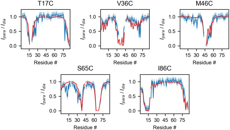
Calculated and experimental PRE HSQC intensity ratios for the T17C, V36C, M46C, S65C and I86C mutants of ACBP.

Blue lines represent the experimental data [53], with the associated ±0.1 error shown by the blue shaded areas. Red lines represent intensity ratios calculated from PDB code 1NTI with τ_c = 2 ns, τ_t = 0.2 ns, t_d = 10 ms, R₂ = 12.6 s⁻¹.

As detailed in S1 Text and S4 Fig, the steric partition functions provided by DEER-PREdict can be used to predict whether a position in the sequence is likely to accommodate the paramagnetic probe within the wild-type structure. Besides aiding the interpretation of experimental data, this feature can be instrumental to designing and enhancing the success-rate of time- and labor-intensive SDSL experiments.

As previously discussed, the explicit treatment of the paramagnetic probe may be crucial for the accurate back-calculation of DEER data, and even more so for PRE predictions, due to the 〈r⁻⁶〉-dependence of the PRE. A common way to restrain MD simulations or to back-calculate PRE experimental data without explicitly simulating the paramagnetic probe is to approximate the electron location to the position of the Cβ atom of the spin-labeled residue [85]. The advantage of this approach is that (a) multiple labeling sites can be analyzed in a single simulation and (b) the explicit atom is present in the simulation making the calculation of PREs straightforward. Cβ-based calculations may, however, be prone to over- or underestimating electron-proton distances by several Å, thereby introducing a systematic error. The impact of the Cβ-approximation on the accuracy of PRE predictions is illustrated in S5 and S6 Figs for the case of ACBP (see also S1 Text).