Mean-field theory with correlations

Consider the problem of linearly mapping a set of correlated inputs x_iμ, with i ∈ 1, …, N and μ = 1, …, P from N_E = f_EN excitatory (E) and N_I = (1 − f_E) inhibitory (I) neurons, onto an output y_μ using a synaptic vector w, in the presence of a learnable constant bias current b (Fig 1). To account for different statistical properties of E and I input rates, we write the elements of the input matrix as $$ {\left(X\right)}_{i\mu }\equiv x_{i\mu }={\overline{x}}_i+{\sigma }_i{\xi }_{i\mu }$$ with $$ {\overline{x}}_i={\overline{x}}_{\text{E}}$$ for i ≤ f_EN and $$ {\overline{x}}_i={\overline{x}}_I$$ for i > f_EN and the same for σ_i. At this stage, the quantities ξ_iμ have unit variance and are uncorrelated across neurons: 〈ξ_iμ ξ_iν〉 = δ_ijC_μν. In the following, we refer to x and y as signals and μ as a time index, although we consider general “semantic”correlations across the patterns x_μ [34]. The output signal has average $$ \langle y_{\mu }\rangle =\overline{y}$$ and variance $$ \langle {(y_{\mu }-\overline{y})}^2\rangle ={\sigma }_y^2$$. We initially consider output signals y_μ with the same temporal correlations as the input, namely 〈δy_μ δy_ν〉 = C_μν, where $$ y_{\mu }=\overline{y}+{\sigma }_y\delta y_{\mu }$$.

Fig 1

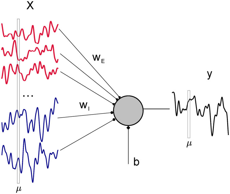
Schematic of the learning problem.

A linear perceptron receives N correlated signals (input rates of pre-synaptic neurons) x_iμ and maps them to the output y_μ through N_E = f_EN excitatory and N_I = (1 − f_E)N plastic inhibitory weights w_i, plus an additional bias current b.

For a given input-output set, we are faced with the problem of minimizing the following regression loss (energy) function:

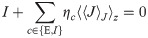
Optimizing with respect to the bias b naturally yields solutions w for which

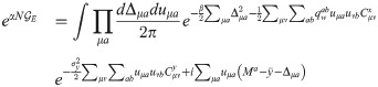
In order to derive a mean-field description for the typical properties of the learned synaptic vector w, we employ a statistical mechanics framework in which the minimizer of E is evaluated after averaging across all possible realizations of the input matrix X and output y. To do so, we compute the free energy density

Critical capacity

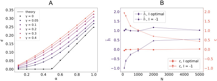
The existence of weight vectors w’s with a certain value of the regression loss E in the error regime (ϵ > 0) is described by the so-called overlap order parameter $$ \Delta {\tilde{q}}_w$$. In the replica-based derivation of the mean-field theory, overlap parameters are introduced with the purpose of decoupling the w_i’s over the i index, and represent the scalar-product of two different configurations of the weights w (Methods: Replica formalism: ensemble covariance matrix (EC)). For finite β, the quantity $$ \Delta q_w=\beta \Delta {\tilde{q}}_w$$ represents the variance of the synaptic weights across different solutions. In the asymptotic limit β → ∞ of Eq (3), a simple saddle-point equation for $$ \Delta {\tilde{q}}_w$$ can be derived when b is chosen to minimize Eq (1):

In the absence of weight regularization (γ = 0), we define the critical capacity α_c as the maximal load α = P/N for which the patterns x_μ can be correctly mapped to their outputs y_μ with zero error. When the synaptic weights are not sign-constrained, the critical capacity is obviously α_c = 1, since the matrix X is typically full rank. In the sign-constrained case, α_c is found to be the minimal value of α such that Eq (4) is satisfied for $$ 0<\Delta {\tilde{q}}_w<+\infty $$. Noting that the left-hand side in Eq (4) is a non-decreasing function of $$ \Delta {\tilde{q}}_w$$ with an asymptote in α, the order parameter $$ \Delta {\tilde{q}}_w$$ goes to + ∞ as the critical capacity is approached from the right. We thus find for γ = 0 the surpisingly simple result:

In [15], the authors showed that, in the case with excitatory synapses only and uncorrelated inputs and outputs, α_c approaches 0.5 in the limit when the quantity $$ \frac{{\sigma }_y^2{\overline{x}}_{\text{E}}^2}{I^2{\sigma }_{\text{E}}^2}$$ goes to zero, and analyzed which conditions on inputs and outputs statistics lead to maximize capacity. Here we take a complementary approach, where the x and y statistics are fixed and capacity is optimized within the error regime, so that the optimal bias $$ I\sqrt{N}$$ is well defined in terms of minimizing 〈E〉 at any load α. The bias optimization leads to a massive simplification of the saddle-point equations and makes results independent of the E/I ratio and the input/output statistics (Methods: EC, Saddle-point equations). One may observe that, in the particular case studied by [15], α_c is maximal for very large I, due to the divergence of the norm of w at critical capacity for an optimal bias in the absence of regularization.

Fig 2

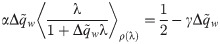
Critical capacity and weight balance.

A: Average loss ϵ for a linear perceptron with f_E = 0.8 positive synaptic weights in the case of i.i.d. input X and output y for increasing values of the regularization γ. Parameters: N = 1000, $$ {\overline{x}}_{\text{E}}={\overline{x}}_I={\sigma }_{\text{E}}={\sigma }_I=\overline{y}={\sigma }_y=1$$. Each point is an average across 50 samples. Full lines show the theoretical results. B: Mean-field component $$ \tilde{h}$$ (left axis, purple) and weight-input correlation c (right axis, red) for increasing dimension N in the case where the bias current $$ b=I\sqrt{N}$$ is either learned (I optimal) or fixed at the outset (I = −1) for f_E = 1, γ = 0.1, α = 0.8. Inputs X and output y are time-correlated with un-normalized Gaussian covariance C, τ = 10 (see text). The remaining parameters are as in A. The asymptotic value $$ \tilde{h}=\overline{y}=1$$ is highlighted by the purple dotted line, the value c = 0 by the red dotted line as guide for the eye.

The independence of our results with respect to the E/I ratio for an optimal bias current signals a local gauge invariance, as observed by [37, 38] for a sign-constrained binary perceptron. Indeed, calling g_i = sign w_i, we can write the mean-removed output as $$ {\sum }_{i=1}^N{g}_i\left|w_i\right|{\sigma }_i{\xi }_i^{\mu }$$ and redefine the ξ’s as $$ g_i{\xi }_i^{\mu }$$, without changing their occurrence probability. This establishes an equivalence to a linear perceptron with non-negative weights (see [37] for more details), once the mean contribution has been removed. Any residual dependence of α_c or ϵ on external parameters must therefore be ascribed to the volume of weights satisfying Eq (2), for a sub-optimal external current b.

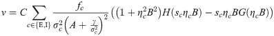
For a generic value of the bias current b, there are strong deviations from the condition in Eq (2). In Fig 2B, we compare the value of the average output $$ \overline{y}$$ with $$ \tilde{h}\equiv {\sum }_{c\in \{\text{E},I\}}{N}_c{\overline{w}}_c{\overline{x}}_c+b$$, and also plot the residual term $$ c=\frac{1}{NP}{\sum }_{i\mu }\delta w_i{x}_{i\mu }$$, where we decomposed the weight vector components as $$ w_i={\overline{w}}_c+\delta w_i$$ for c ∈ {E, I}. The quantity c measures weight-rate correlations that are responsible for the cancelation of the $$ \mathcal{O}\left(\sqrt{N}\right)$$ bias.

The deviation from Eq (2), shown here for a rapidly decaying covariance of the form $$ C_{\mu \nu }=e^{-\frac{|\mu -\nu |}{2{\tau }^2}}$$, has been previously described in the context of a target-based learning algorithm used to build E-I-separated rate and spiking models of neural circuits capable of solving input/output tasks [3]. In this approach, a randomly initialized recurrent network n_T is driven by a low dimensional signal z. Its currents are then used as targets to train the synaptic couplings of a second (rate or spiking) network n_S, in such a way that the desired output z can later be linearly decoded from the self-sustained activity of n_S. Each neuron of n_S has to independently learn an input/output mapping from firing rates x to currents y, using an on-line sign-constrained least square method. In the presence of an L2 regularization and a constant $$ b\propto \sqrt{N}$$ external current, the on-line learning method typically converges onto a solution for the recurrent synaptic weights for which Eq (2) does not hold. As also shown in [3], in the peculiar case of a self-sustained periodic dynamics (in which case off-diagonal terms of the covariance matrix C_μν do not vanish for large μ or ν) the two contributions $$ \tilde{h}$$ and c scale approximately like $$ \sqrt{N}$$ and cancel each other to produce an $$ \mathcal{O}\left(1\right)$$ total average output $$ \overline{y}=\tilde{h}+c$$. In the effort to build heterogeneous functional network models, the emergence of synaptic connectivity compatible with the balanced scaling thus depends on the statistics of incoming currents. Ad-hoc regularization can be avoided by adjusting external currents onto each neuron.

Power spectrum and synaptic distribution

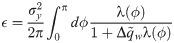
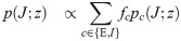
The theory developed thus far applies to a generic covariance matrix C. To connect the spectral properties of C with the signal dynamics, we further assume the x_iμ to be N independent stationary discrete-time processes. In this case, C_μν = C(μ − ν) is a matrix of Toeplitz type [39], leading to the following expression for the average minimal loss density in the N → ∞ limit:

Fig 3

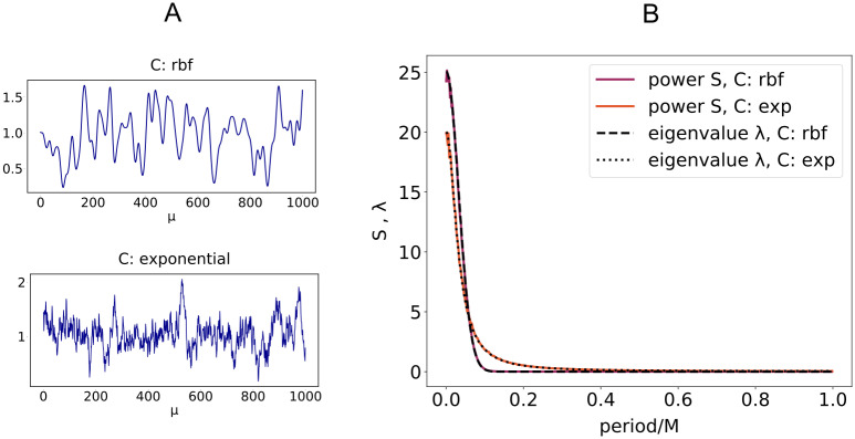
Eigenvalues of C and Fourier spectrum.

A: Examples of excitatory input signals x_iμ (i ∈ E) with two different covariance matrices C. Top: rbf covariance, τ = 10. Bottom: exponential covariance $$ C_{\mu \nu }=e^{-\frac{|\mu -\nu |}{\tau }}$$, τ = 10. Parameters: $$ {\overline{x}}_{\text{E}}=1$$, σ_E = 0.3. B: Theoretical eigenvalue spectrum of C with τ = 10 versus average power spectrum for positive wave numbers across N = 2000 independent processes with P = 1000 time steps.

As shown in Fig 4A in the case of input x and output y with rbf covariance, the squared norm of the optimal synaptic vector w (red curve) is in general a non-monotonic function of α, its maximum being attained at bigger values of α as the time constant τ increases. We also show the minimal loss density ϵ and the mean error ϵ_err for γ = 0.1. The curves in Fig 4A are the same for any ratio f_E: the use of an optimal bias current b cancels any asymmetry between E and I populations. For a finite γ, the minimal average loss ϵ for a given f_E decreases as either σ_E or σ_I increase. For a given set of parameters f_E and γ, the optimal bias b will in general depend on the load α and the structure of the covariance matrix C, as shown in Fig 4B.

Fig 4

Learning temporally structured signals.

A: Minimal loss ϵ, error ϵ_err and norm of the weight vector w as a function of the load α for a linear perceptron trained on a time-correlated signal. Covariance matrix C is of rbf type with τ = 2. Parameters: N = 1000, f_E = 0.8, γ = 0.1, $$ {\overline{x}}_{\text{E}}={\overline{x}}_I={\sigma }_{\text{E}}={\sigma }_I=\overline{y}={\sigma }_y=1$$. B: Optimal bias b for the two sets of signals with rbf (black curve) and exponential (yellow curve) covariance C, with τ = 2. Theoretical curves show the value $$ I\sqrt{N}+\overline{y}$$, where I has been computed from the saddle-point equations (Methods: EC, Saddle-point equations). Parameters as in A. Each point in A and B is an average across 50 samples. C: Probability density of non-zero synaptic weights $$ w_i\sqrt{N}$$ of a linear perceptron with N = 1000, a fraction f_E = 0.8 of excitatory weights, trained on P = 600 exponentially correlated input x and output y. The δ function in zero is omitted for better visualization. Parameters: τ = 10, γ = 0.1, $$ {\overline{x}}_{\text{E}}={\overline{x}}_I=1$$, σ_I = 2σ_E = 0.4. The histogram is an average across 50 realizations of input/output signals. Inset: full histogram of synaptic weights $$ w_i\sqrt{N}$$.

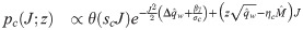
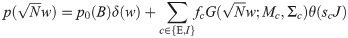
Using the same analytical machinery employed for the calculation of the free energy Eq (3), the probability distribution of the typical weight w_i can be easily derived. This can be seen by employing a variant of the replica trick (Methods: Distribution of synaptic weights) that links the so-called entropic part of f to 〈p(w_i)〉, expressed in terms of the saddle-point values of the same (conjugated) overlap parameters employed thus far. Interestingly, the optimal bias b implies that half of the synapses are zero, irrespectively of f_E and the properties of the covariance matrix C. The probability density of the synaptic weights is composed of two truncated Gaussian densities with zero mean for the E and I components, plus a finite fraction p₀ = 0.5 of zero weights.

We show in Fig 4C the shape of the optimal weight distribution for a linear perceptron with 80% excitatory synapses, trained on exponentially correlated x and y and with a ratio σ_I/σ_E = 2. It is interesting to note that, in the presence of an optimal external current, both the means of the Gaussian components and the fraction of silent synapses do not depend on the specific properties of input and output signals.

The shape of the synaptic distribution appeared in previous studies both in the binary [8, 11, 13] and linear perceptron [15]. In the linear case with only excitatory synapses [15], for a fixed bias $$ b=\sqrt{N}$$, the fraction of zero E weights is larger than 0.5 at criticality. It generally depends on input parameters and the load in the error region α ≤ α_c. Let us also mention that a similar property is also apparent in the binary perceptron, where the scale of the typical solutions is set by robustness [13] to input and output noise. For weights $$ w_i=\mathcal{O}(1/\sqrt{N})$$, the sparsity of critical solutions generically depends on properties of E and I inputs. For weights of $$ \mathcal{O}(1/N)$$, robust solutions have a fraction of zero E weights generically larger than 0.5 [6, 11]. When inhibitory synapses are added, their weights are less sparse [11]. Interestingly, in the case without robustness, half of the E and I weights are zero at critical capacity for all f_E ≥ 0.5.

The dynamic properties of input/output mappings affect the shape of the weight distribution in a computable manner. As an example, in a linear perceptron with non-negative synapses, the explicit dependence of the variance of the weights on the input and output auto-correlation time constant is shown in Fig 5A for various loads α. Previous work considered an analog perceptron with purely excitatory weights as a model for the graded rate response of Purkinje cells in the cerebellum [15]. In the presence of heterogeneity of synaptic properties across cells, a larger variance in their synaptic distribution is expected to be correlated with high frequency temporal fluctuations in input currents. Analogously, the auto-correlation of the typical signals being processed sets the value of the constant external current that a neuron must receive in order to optimize its capacity.

When the input and output have different covariance matrices C^x ≠ C^y, a joint diagonalization is not possible in general (Methods: EC, Energetic part). We can nevertheless write an expression (Eq (23)) that holds when input and output patterns are defined on a ring (with periodic boundary conditions) and use it as an approximation for the general case. Fig 5B shows good agreement between numerical experiment and theoretical predictions for the error ϵ_err and the squared norm of the synaptic weight vector w, when input and output processes have two different time-constants τ_x and τ_y.

Fig 5

Input/Output time constants and learning performance.

A: Variance of synaptic weights (f_E = 1) for a linear perceptron of dimension N = 1000 trained on rbf-correlated signals with increasing time constant τ for three different values of the load α. Parameters: γ = 0.1, $$ {\overline{x}}_{\text{E}}={\overline{x}}_I={\sigma }_{\text{E}}={\sigma }_I=\overline{y}={\sigma }_y=1$$. B: Average error ϵ_err in the case where input and output signals have two different covariance matrices, for increasing time constant τ_y of the output signal y. Parameters: N = 1000, f_E = 0.8, γ = 0.1, $$ {\overline{x}}_{\text{E}}={\overline{x}}_I=\overline{y}={\sigma }_y=1$$, σ_I = 2σ_E = 0.6, C^x rbf with τ_x = 1, C^y rbf with various values of τ_y. Inset: norm of the weight vector w. Full lines show analytical results. Points are averages across 50 samples.

Sample covariance and dimensionality

In the discussion thus far, we assumed independence across the “spatial” index i in the input. It is often the case for input signals to be confined to a manifold of dimension smaller than N, a feature that can be described by various dimensionality measures, some of which rely on principal component analysis [40, 41]. In order to relax the independence assumption, we build on a framework originally introduced in the theory of spin glasses with orthogonal couplings [42–44] and further developed in the context of adaptive Thouless-Anderson-Palmer (TAP) equations [45–47]. In the TAP formalism, a set of mean-field equations is derived for a given instance of the random couplings (in our case, for a fixed input/output set). In its adaptive generalization [46], the structure of the TAP equations depends on the specific data distribution, in such a way that averaging the equations over the random couplings yields the same results of the replica approach. Here, following previous work in the context of information theory of linear vector channels and binary perceptrons [48–51], we employ an expression for an ensemble of rectangular random matrices and use the replica method to average over the input X and output y.

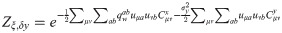
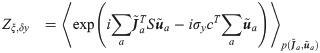
Let us write the input matrix $$ {\left(X\right)}_{i\mu }={\overline{x}}_i+{\sigma }_i{\xi }_{i\mu }$$, with ξ = USV^T, S being the matrix of singular values. To analyze the properties of the typical case, we start from a generic singular value distribution S and consider i.i.d. output y_μ. In calculating the cumulant generating function Z_ξ,δy, we perform a homogeneous average across the left and right principal components U and V (Methods: SC, Energetic part). Calling ρ_ξξ^T(λ) the eigenvalue distribution of the sample covariance matrix ξξ^T, we can express Z_ξ,δy in terms of a function $$ {\mathcal{G}}_{\xi ,\delta y}$$ of an enlarged set of overlap parameters, which depends on the so-called Shannon transform [52] of ρ_ξξ^T(λ), a quantity that measures the capacity of linear vector channels. The resulting self-consistent equations, which describe the statistical properties of the synaptic weights w_i, are expressed in terms of the Stieltjes transform of ρ_ξξ^T(λ), an important tool in random matrix theory [53] (Methods: SC, Saddle-point equations).

We show the validity of the mean-field approach by employing two different data models for the input signals. In the first example, valid for α ≤ 1, all the P vectors ξ_μ are orthogonal to each other. This yields an eigenvalue distribution of the simple form ρ(λ) = αδ(λ − 1) + (1 − α)δ(λ), for which the function $$ {\mathcal{G}}_{\xi ,\delta y}$$ can be computed explicitly [51]. Additionally, we use a synthetic model where we explicitly set the singular value spectrum of ξ to be $$ s\left(\alpha \right)=\chi e^{-\frac{{\alpha }^2}{2{\sigma }_x^2}}$$, with χ a normalization factor ensuring matrix ξ has unit variance. The shape of the singular value spectrum s controls the spread of the data points ξ_μ in the N-dimensional input space, as shown in Fig 6A. As shown in Fig 6B for i.i.d Gaussian output, learning degrades as σ_x decreases, since inputs tend to be confined to a lower dimensional subspace rather than being equally distributed along input dimensions.

Fig 6

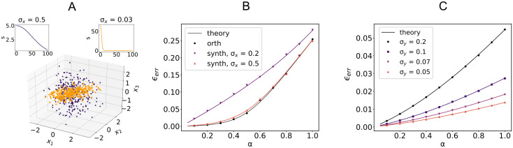
Sample-based PCA and learning performance.

A: First three components of inputs ξ_μ with Gaussian singular value spectrum s for two different values of σ_x (color coded top panels). Parameters: N = 100, P = 300. B: Average error ϵ_err for three different singular value spectra of the input sample covariance matrix: orthogonal model and Gaussian model with increasing σ_x (see main text for definition of σ_x). Outputs are i.i.d Gaussian. Parameters: N = 1000, f_E = 0.8, γ = 0.1, $$ {\overline{x}}_{\text{E}}={\overline{x}}_I=\overline{y}={\sigma }_y=1$$, σ_I = 2σ_E = 0.6. B: Average error ϵ_err for input with orthogonal-type covariance and output y with rbf-type covariance with decreasing σ_y (see main text for the definition of σ_y). All remaining parameters as in A. Full lines show analytical results. Points are averages across 50 samples.

For N large enough (in practice, for N ≳ 500), the statistics of single cases is well captured by the equations for the average case (self-averaging effect). To get a mean-field description for a single case, where a given input matrix X is used, we further assume we have access to the linear expansion c_μ of the output y in the set {v_μ} of the columns of the V matrix, namely $$ y=\overline{y}+{\sigma }_{y}Vc$$. The calculation can be carried out in a similar way and yields, for the average regression loss, the following result:

In Fig 6C, we show results when the dimensionality of the output y along the (temporal) components of the input is modulated by taking $$ c\left(\alpha \right)=e^{-\frac{{\alpha }^2}{2{\sigma }_y^2}}$$. The perceptron performance improves as the output signals spreads out across multiple components v_μ. The case of i.i.d. output is recovered by taking c_μ = 1.

Replica formalism: Ensemble covariance matrix (EC)

Using the Replica formalism [67], the free energy density is written as:

To simplify the formulas, we introduce the $$ \mathcal{O}\left(1\right)$$ weights $$ J_i={\sigma }_i\sqrt{N}{w}_i$$. In terms of these rescaled variables, the loss function in Eq (1) takes the form:

EC, Entropic part

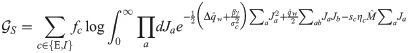
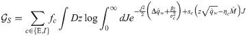
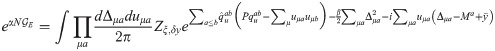
The total volume of configurations w_a for fixed values of the overlap parameters is given by the entropic part:

where we called $$ {\eta }_c=\frac{{\overline{x}}_c}{{\sigma }_c}$$, with c ∈ {E, I}, and η_i = η_E (η_i = η_I) if i ∈ E (i ∈ I). Using the RS ansatz $$ {\widehat{q}}_w^{ab}={\widehat{q}}_w-{\delta }_{ab}\frac{{\widehat{q}}_w+\Delta {\widehat{q}}_w}{2}$$ and $$ {\widehat{M}}^a=\widehat{M}$$, we get:

Using the explicit definition of the measure $$ d\mu \left(J\right)\propto {\prod }_{i\in \text{E}}\theta \left(J_i\right)d{J}_i{\prod }_{k\in I}\theta (-J_k)d{J}_k$$, one has, up to constant terms:

where we introduced the notations f_I = 1 − f_E and s_E = −s_I = 1. In order to disentangle the term ∑_ab J_aJ_b = (∑_a J_a)², we employ the so-called Hubbard-Stratonovich transformation $$ e^{\frac{b^2}{2}}=\int Dz{e}^{bz}$$, where $$ Dz=dz\frac{e^{-\frac{z^2}{2}}}{\sqrt{2\pi }}$$. Taking the limit n → 0 one gets:

EC, Energetic part

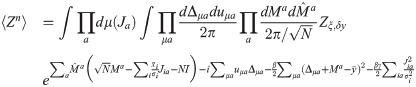
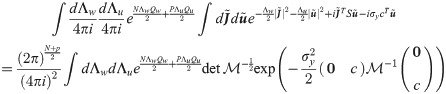
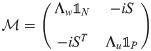
In order to compute the energetic part, we first need to evaluate the average with respect to ξ and δy in Eq (11). Performing the two Gaussian integrals we get:

from which:

where we performed a translation $$ {\Delta }_{\mu a}+M^a-\overline{y}\to {\Delta }_{\mu a}$$. In the special case C^x = C^y ≡ C, we can use C = VΛV^T to jointly rotate Δ_a → V Δ_a and u_a → Vu_a, thus leaving scalar products invariant. By doing so, we obtain, within the RS ansatz:

where ζ_μ = ∑_ν V_μν. Using a Hubbard-Stratonovich transformation on the term ∑_ab u_μa u_μb, after some algebra, we obtain:

Observing that the free energy only depends on M through the term $$ {(M-\overline{y})}^2$$ in $$ {\mathcal{G}}_E$$, we conveniently eliminate the quantities ζ_μ at this stage, using the simple saddle-point relation

thus getting:

The brackets 〈⋅〉_λ in Eq (22) stand for an average over the eigenvalue distribution ρ(λ) of C in the N → ∞ limit, assuming self-averaging. A similar expression for $$ {\mathcal{G}}_E$$ was previously derived in [34] for spherical weights, i.e. $$ {\sum }_{i=1}^N{w}_i^2=1$$, in the presence of outputs y_μ generated by a teacher linear perceptron. To map Eq (45) in [34] to Eq (22), one substitutes (1 − q) → Δq_w (observing that q^aa = 1 thanks to the spherical constraint) and sets R = 0, since the learning task only involves patterns memorization.

When C^x ≠ C^y, we can derive a similar expression under the assumption of a ring topology in pattern space (corresponding to periodic boundary conditions in the index μ): in this case, both covariance matrices are circulant and may be jointly diagonalized by discrete Fourier transform [33, 34]. In the main text, we show that the expression

yields good results also when C^x and C^y are covariance matrices of stationary discrete-time processes.

EC, Saddle-point equations

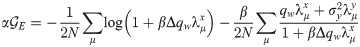
All in all, the free energy density in the saddle-point approximation is:

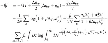
The saddle-point equations stemming from the entropic part can be written as:

where the averages 〈⋅〉_J and 〈⋅〉_z in Eqs (25)–(27) are taken with respect to the mean-field distribution of the J weights:

where z is a standard normal variable and θ is the Heaviside function: θ(x) = 1 when x > 0 and 0 otherwise. Eq (25) is obtained by differentiating Eq (24) with respect to $$ {\widehat{q}}_w$$ and then performing an integration by part in z. Eq (26) is easily obtained by subtracting Eq (25) from the saddle-point condition over $$ \Delta {\widehat{q}}_w$$, while Eq (27) originates from the derivative w.r.t. $$ \widehat{M}$$.

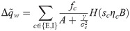
In the β → ∞ limit, the unicity of solution for γ > 0 implies that Δq_w → 0. We therefore use the following scalings for the order parameters:

while $$ q_w=\mathcal{O}\left(1\right)$$. In this scaling, Eqs (25)–(27) take the form:

where $$ G\left(x\right)=\frac{e^{-\frac{x^2}{2}}}{\sqrt{2\pi }}$$ and $$ H\left(x\right)={\int }_x^{\infty }Dz$$. The two remaining saddle-point equations are:

Optimizing f with respect to the bias $$ b=I\sqrt{N}$$ immediately implies B = 0, by virtue of Eq (33), and greatly simplifies the saddle-point equations. Using the scaling assumptions Eqs (30)–(33) together with the saddle-point Eqs (34)–(38), we get Eq (4) in the main text, that is valid for any α for γ > 0. In the unregularized case (γ = 0), it describes solutions in the error regime α > α_c. The optimal bias b can be computed by $$ I\sqrt{N}$$ using Eq (36), that is valid up to an $$ \mathcal{O}\left(1\right)$$ term equal to $$ \overline{y}$$ (Fig 4B). Keeping only the leading terms in the limit β → ∞, Eq (24) can be written as:

From the definition of the free energy density −βNf = 〈log∫dμ(w)e^−βE〉, one has that $$ \frac{\langle E\rangle }{N}={\partial }_{\beta }\left(\beta f\right)$$. Using Eq (39) and the relevant saddle-point equations, the expression for the average minimal energy density is then:

Also, noting that $$ {\partial }_{\gamma }E=\frac{N}{2}{\sum }_{i=1}^N{w}_i^2$$, we can compute the average squared norm of the weights $$ v={\sum }_{i=1}^N\langle w_i^2\rangle $$ by v = 2∂_γ f. We thus obtain:

The error $$ {ϵ}_{err}=\frac{1}{2N}\langle {|X^T\mathit{w}+\mathit{b}-\mathit{y}|}^2\rangle $$ can be then computed by $$ {ϵ}_{err}=ϵ-\frac{\gamma }{2}v$$.

Distribution of synaptic weights

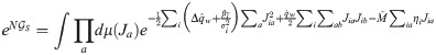
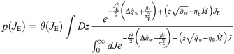
The synaptic weight distribution appearing in Eqs (28) and (29) can be obtained using a variant of the replica trick [6, 67]. Using the expression Z⁻¹ = lim_{n → 0} Zⁿ⁻¹, the density of excitatory weights can be written as:

Spectrum of exponential and rbf covariance

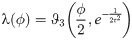
For the exponential covariance $$ C_{\mu \nu }=e^{-\frac{|\mu -\nu |}{\tau }}$$, one has [33]:

Replica formalism: Sample covariance matrix (SC)

Also in the case of a sample covariance matrix, we are interested in statistically structured inputs and output. An independent average across x and y would result in a simple dependence on the variance of y in the energetic part. To capture the geometric dependence between x and y, we thus extend the calculations in [50, 51] to the case where the linear expansion of y_μ on the right singular vectors V_⋅μ is known, by taking δy_μ = ∑_ν V_μν c_ν.

In order to compute the replicated cumulant generating function Eq (11), we again introduce overlap parameters $$ q_w^{ab}$$, whose volume is given by the previously computed entropic part $$ {\mathcal{G}}_S$$. The fact that the entropic part is unchanged in turn implies that the mean-field weight distribution takes the form of Eq (44), with the values of {A, B, C} being determined by a new set of saddle-point equations.

SC, Energetic part

Using again the expressions $$ {\left(X\right)}_{i\mu }={\overline{x}}_i+{\sigma }_i{\xi }_{i\mu }$$ and ξ = USV^T, the replicated cumulant generating function for the joint (mean-removed) input and output is:

where we used the change of variables $$ {\tilde{J}}_{ia}={\sum }_k{U}_{ki}{J}_{ka}$$ and $$ {\tilde{u}}_{\mu a}={\sum }_k{V}_{k\mu }{u}_{ka}$$. The average in Eq (47) is taken over the joint distribution $$ p({\tilde{\mathit{J}}}_a,{\tilde{\mathit{u}}}_a)$$ resulting from averaging over the Haar measure on the orthogonal matrices U and V. For a single replica, Z_ξ,δy will only depend on the squared norms $$ Q_w={\sum }_i\frac{{\tilde{J}}_i^2}{N}$$ and $$ Q_u={\sum }_{\mu }\frac{{\tilde{u}}_{\mu }^2}{P}$$ of the two vectors $$ \tilde{\mathit{J}}$$ and $$ \tilde{\mathit{u}}$$. We can therefore write the average in the following way:

Introducing Fourier representation for the δ functions, we are left with an expression involving an N + P dimensional Gaussian integral:

where

and $$ {\mathbb{1}}_K$$ is the identity matrix of dimension K. Following [51], the determinant can be easily calculated:

where the limit is taken for N → ∞ and the average is with respect to the eigenvalue distribution ρ(λ^x). As for the quadratic portion of the Gaussian integral, calling $$ {\lambda }_k^y=c_k^2$$, we will use the shorthand

Considering now the replicated generating function, all the n(n + 1) cross-product $$ {\mathit{J}}_a·{\mathit{J}}_b={\tilde{\mathit{J}}}_a·{\tilde{\mathit{J}}}_b$$ and $$ {\mathit{u}}_a·{\mathit{u}}_b={\tilde{\mathit{u}}}_a·{\tilde{\mathit{u}}}_b$$ must be conserved via the multiplication of U and V. Together with the overlap parameters $$ N{q}_w^{ab}={\sum }_i{J}_{ia}{J}_{ib}$$, we additionally introduce the quantities $$ P{q}_u^{ab}={\sum }_{\mu }{u}_{\mu a}{u}_{\mu b}$$, thus obtaining:

In the RS case, we again take $$ q_w^{ab}=q_w+{\delta }_{ab}\Delta q_w$$ and, similarly for the u’s, $$ q_u^{ab}=-q_u+{\delta }_{ab}\Delta q_u$$. In the basis where both $$ q_w^{ab}$$ and $$ q_u^{ab}$$ are diagonal, the expression for Z_ξ,δy becomes

so, calling $$ {\mathcal{G}}_{\xi ,\delta y}=\frac{1}{N}{\text{lim}}_{n\to 0}\text{log}{Z}_{\xi ,\delta y}$$, we have:

with the function F given by:

and $$ K({\Lambda }_w,{\Lambda }_u)={\Lambda }_w{\langle \frac{{\lambda }^y}{{\lambda }^x+{\Lambda }_w{\Lambda }_u}\rangle }_{{\lambda }^x,{\lambda }^y}$$. In Eq (54), it is intended that Λ_w and Λ_w are implied by the Legendre Transform conditions:

The remaining terms in the energetic part $$ {\mathcal{G}}_E$$ involve the $$ q_u^{ab}$$ overlaps and their conjugated parameters $$ {\widehat{q}}_u^{ab}$$. Introducing the RS ansatz $$ {\widehat{q}}_u^{ab}={\widehat{q}}_u+{\delta }_{ab}\frac{\Delta {\widehat{q}}_u-{\widehat{q}}_u}{2}$$, the calculation follows along the same lines of the section SC, Energetic part. We get:

Eliminating M, $$ {\widehat{q}}_u$$ and $$ \Delta {\widehat{q}}_u$$ at the saddle-point in Eq (58), $$ {\mathcal{G}}_E$$ reduces to:

SC, Saddle-point equations

The final expression for the free energy density

implies the following saddle-point equations:

in addition to the entropic saddle-point Eqs (25)–(27), which are unchanged. The saddle-point values of the conjugate Legendre variables Λ_w, Λ_u greatly simplify the expression for the first and second derivatives of F. Indeed, from Eqs (61) and (62) one has:

or, setting $$ {\Lambda }_w=\beta {\tilde{\Lambda }}_w$$:

In particular, Eq (56) shows that $$ \Delta {\tilde{q}}_w$$ is expressed by a Stieltjes transform of ρ(λ^x) and the first term in Eq (55) is its Shannon transform. In the limit β → ∞, using the following additional scaling relations for the u overlaps:

we get the expression for the energy density:

SC, i.i.d. and unconstrained cases

Either setting K = 0 or λ^y = 0 reverts back to the i.i.d. output case. In the special case of i.i.d. inputs, the eigenvalue distribution is Marchenko-Pastur

with $$ {\lambda }_{+/-}={(1\pm \sqrt{\alpha })}^2$$, from which $$ F(\Delta q_w,\Delta q_u)=-\frac{\alpha }{2}\Delta q_w\Delta q_u$$. The saddle-point equations are essentially the same as the ones in the section EC, Saddle-point equations with $$ C_{\mu \nu }^x=C_{\mu \nu }^y={\delta }_{\mu \nu }$$.

Let us also note that, in the simple unconstrained case, taking for simplicity $$ {\overline{x}}_i=0$$ and b = 0, the entropic part can be worked out to be, up to constant terms:

which, at the saddle-point, implies $$ {\tilde{\Lambda }}_w=\gamma $$. The mean-field distribution $$ p\left(\sqrt{N}w\right)$$ is a zero-mean Gaussian with variance v = q_w. Using the properties of the Hessian of the Legendre Transform, it is easy to show that:

These expressions can also be derived from the pseudo-inverse solution (we take $$ \overline{y}=0$$ for simplicity) w* = (ξξ^T + γ)⁻¹ ξy, by taking an average across ξ and y in the two expressions:

The i.i.d. output case also follows by performing independent averages over y and ξ.