Data preparation

We used a subset of a global collection of ∼19,000 Mtb samples with whole-genome sequencing data from which ∼600,000 SNPs were derived [10] (see the ‘Additional file 2’ in ref. [10] for a list of accession codes and references). In brief, raw sequence data were mapped to the H37Rv reference genome with bwa-mem. From the alignments, variants were called using the GATK and samtools [27] software suites. Because we wished to focus on virulent strains and reduce the size of dataset (non-synonymous SNPs constituted less than half of all called variants), all Beijing strains (n = 3,574) and their polymorphic missense SNPs (41,319) were selected. Alleles were converted into binary genotypes, where ‘0’ represents the reference genotype and ‘1’ a missense-SNP at the respective genomic position. To check for biases in the missense SNPs versus the unfiltered Beijing dataset, the corresponding distributions of variants, allele counts and missing genotypes were plotted and principal component analysis (PCA) was performed on both matrices.

Although the dataset contained categorical resistance data for 15 antibiotics, most strains had only been phenotyped for the most common first-line drugs. Hence, this work only considered INH, RIF, EMB, PZA, and SM. Strains with known resistance status for at least one of these five drugs were selected for analysis. Each of the resulting six datasets (one per drug and one including all drugs) was filtered to remove SNPs and samples with more than 10% uncalled genotypes as well as mono-allelic sites. For all analyses intolerable to missing data the corresponding genotypes were set to the respective allele frequency.

Strain metadata including resistance status to the five drugs are available in S6 Data. The filtered genotype matrix can be found in S7 Data.

Phylogenomics

A phylogenetic tree was obtained from the ∼41,000 missense SNPs using fasttree (v2.1.11) [28] with a Generalised Time Reversible (GTR) substitution model and branch length rescaling to optimise the Gamma20 likelihood. The multi-FASTA alignment file required for running fasttree was generated from the called variants using vcf2phylip (v2.0) [29]. A proto-Beijing strain (ERR751993) belonging to lineage 2.1 was presented as the outgroup. The resulting tree topology was then evaluated under various model parameters with RAxML-NG (v0.9.0) [30] (the evaluation step re-optimises the branch lengths under a given model). For all subsequent analyses requiring phylogenetic input, the tree with the lowest AIC metric [31] was used. It was created using GTR with the Gamma model for rate heterogeneity and estimated base frequencies. The tree was visualised with ggtree (v1.16.3) [32]. The command line arguments used for fasttree and RAxML-NG are listed in S1 Methods.

Genome-wide association studies

GWAS was performed with multiple ways of correcting for population structure, including multidimensional scaling (MDS) as implemented in SEER [16], linear mixed models as in FaST-LMM [17] and lineage effects as in bugwas [15]). These analyses were run via the pyseer package [33]. SEER was run once with four and once with ten dimensions to be included in MDS. The pairwise distance as well as similarity matrices were generated from the phylogenetic tree by the respective scripts coming with pyseer. Homoplastic variants were tested for convergent evolution with treeWAS [13]. We provided the phylogenetic tree employed in the analysis, whereas the ancestral reconstruction was performed by treeWAS internally. The command line arguments passed to SEER can be found in S1 Methods.

Statistical and machine learning

Most ML methods employed were available via Python’s sklearn package (v0.21.2) [34]. These included regularised linear regression (L1 penalised; i.e. Lasso [35]), logistic regression (L1 and L2 penalised), support vector machines [SVMs; using linear and radial basis function (RBF) kernels] [36], decision trees [37], random forests [38], and gradient boosted decision trees [39]. Neural networks (NNs) were implemented with Keras (v2.2.4) [40] upon TensorFlow (v1.13.1) [41]. Model parameters are described in more detail in S2 Methods and the NN architecture is illustrated in S1 Fig.

All algorithms were applied on the five single-drug datasets separately. Additionally, an extra NN was trained for multi-label classification on the dataset with all drugs. Thus, it would predict resistance against one or more of the five drugs simultaneously. Each dataset was split into training and testing batches stratified for phenotype at a ratio of 0.7 to 0.3. The models were then trained on the training data and benchmarked on the testing data. During training of the NNs, 20% of the training data were used for validation. For selecting the optimal shrinkage parameters for Lasso and logistic regressions, sklearn’s respective cross-validation functions were utilised. Decision trees were left at default parameters (representing minimum restriction) or constrained to a maximum depth of five. Hyperparameters for random forests and gradient boosted trees were selected with sklearn’s cross-validated grid-search method according to the F₁-score [42] as scoring metric. Class weights were balanced wherever possible.

For Lasso and linear SVM the absolute magnitude of model coefficients was interpreted as feature importance. For logistic regression, a likelihood-ratio test was implemented [43, 44]. The test calculates two p-values for a given feature according to two different approaches: (i) the corresponding regression coefficient is set to zero and the resulting difference in log-likelihood of the prediction of the training set is subjected to a χ² test; (ii) the model is fit on the respective feature alone and the difference of the prediction log-likelihood to the raw class probabilities is subjected to a χ² test. p-values were calculated for the 1000 features with the largest absolute regression coefficients per model.

For all other sklearn models (except for SVM with RBF kernel) feature importance values were determined by the respective implementation internally. From NNs or SVMs with non-linear kernels feature importance cannot be quantified directly, but must be estimated by monitoring prediction accuracy while permuting the input data [45]. However, this requires predicting a considerable number of samples at least once per feature and thus is computationally infeasible given the size of the datasets used in this work.

Hungry, Hungry SNPos algorithm (HHS)

To minimise the confounding effects of co-occurrent resistance markers, we formulated an iterative, ‘cannibalistic’ elimination algorithm. In its first stage an initial score for each SNP i is calculated according to

The rationale behind this formulation as opposed to the scores calculated by treeWAS is that p¹ g⁰ and p⁰ g⁰ add little relevant information for assessing a particular variant as resistance in strains with p¹ g⁰ could be caused by other SNPs (which we did not want to penalise) and because p⁰ g⁰’s relation to a SNP’s association with resistance is typically weak. p¹ g¹ favours high-frequency alleles in imbalanced datasets with a large proportion of resistant strains, but this can be counteracted by a sufficiently high w_p⁰g¹. In the actual implementation, additional weights can be applied to normalise for the overall allele frequency at the respective site and class imbalance in the phenotype. The weight of the distance d_{p¹g¹, i} is tunable as well. See S3 Methods for a more detailed description of the different parameters.

After this first step all SNPs with positive scores are subjected to iterative elimination as outlined in S3 Methods. In every iteration, the procedure reduces the score of every SNP i by an amount that is proportional to (i) the overlap of i with other SNPs across all resistant strains and (ii) the magnitude of these other SNPs’ scores. After each iteration, all scores are rescaled so that their overall sum stays the same. Thus, some scores will grow and others will shrink. As soon as a score drops below zero, it is no longer considered. After a certain number of iterations, a stable set of SNPs remains.

The results reported below were generated with a Python prototype relying on NumPy [46, 47], SciPy [48], pandas [49], and Numba [50]. First, the pairwise Hamming distances between all strains in the dataset were calculated. Then, HHS was run on the five single-drug datasets in various different configurations (for details see S3 Methods) for 20,000 iterations each. This was enough to let the algorithm converge (i.e. the scores would no longer change). A Rust [51] implementation optimised for memory efficiency (with a footprint of $$ \sim 1/4\times n_{\text{samples}}\times n_{\text{SNPs}}+2\times n_{\text{samples}}^2$$ bytes) is available at https://github.com/julibeg/HHS. A run of 20,000 iterations (e.g. to test a specific set of parameters) with the Beijing dataset took about 20 seconds (or 10, if the pairwise distances were already known) on a standard laptop, whereas hours of high-performance computing were required for some of the other methods tested herein.

Mtb Beijing strain data and phylogeny

The Beijing strains (n = 3,574) were from 43 countries, with nearly half (n = 1771; 49.6%) from Thailand, South Africa and Russia (S2 Fig). To check for systematic biases within the set of missense SNPs, the distributions of variants, non-calls and allele-counts were compared with the original dataset holding all SNPs and no striking differences were found (S3 and S4 Figs).

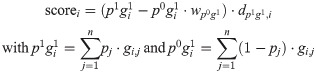
For each of the five drugs, sample sizes varied from 1489 (SM) to 3547 (RIF), leading to between 24,946 and 41,040 SNPs being analysed, respectively (Table 1). The differences are driven by the number of susceptibility tests performed for each drug across the 3,574 samples (Fig 1, top). There is a high level of co-occurring resistance, especially between partner drugs such as INH and RIF, leading to a high proportion of the samples being MDR-TB (Fig 1, bottom). This makes detecting resistance-conferring SNPs difficult as mutations strongly associated with resistance to one drug (e.g. katG S315N/T for INH) also give large association signals when analysing other drugs.

Fig 1

Distribution of resistance phenotypes.

Top: Bar plot of resistant, susceptible and missing phenotypes per drug. Bottom: Pairwise co-occurring resistance for the five drugs in the dataset. Colours are relative to the drug with fewer resistant strains (e.g. 597/659 = 0.906 for SM and INH, 1072/1115 = 0.961 for EMB and RIF etc.). The upper triangle of the symmetric matrix has been removed for clarity.

Table 1

Specifics of the datasets used.

Dataset	N	% resistant	Training N	Testing N	SNPs
All drugs	3574	60.9	2501 (501)	1073	41319
INH	3501	55.5	2450 (490)	1051	41040
RIF	3547	52.8	2482 (497)	1065	41120
EMB	3352	33.3	2346 (470)	1006	40252
PZA	2212	31.4	1548 (310)	664	22403
SM	1489	44.3	1042 (209)	447	24946

The size of the respective training subset used for validation in neural net hyperparameter search is given in brackets. N, number of samples.

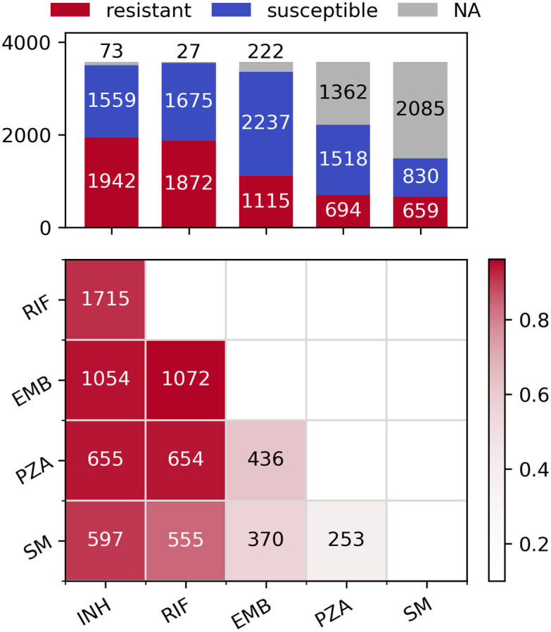
A phylogenetic tree inferred from the 41,319 missense SNPs revealed that the XDR strains clustered relatively well, with evidence of potential transmission clusters for single countries (South Africa and Belarus; Fig 2). Otherwise, samples with the same resistance status or that originated from the same country spread throughout the tree. This was also found in a PCA (S5 Fig), with the majority of clusters being heterogeneous.

Fig 2

Phylogeny of the dataset.

Tracks are coloured by resistance status (inner track) and source country of Mtb (outer track). The root node was omitted for clarity.

Resistance mutations found using GWAS and phylogeny testing

The four SNPs most significantly associated with each drug as determined by GWAS with FaST-LMM are presented in Table 2. Similarly, the significant SNPs for SEER are listed in S1 and S2 Tables. The results produced by FaST-LMM featured the least number of co-resistant false positives, which might be attributed to it being less prone to inflating p-values as opposed to SEER [52]. The SEER results showed only minimal difference between projecting the phylogenetic distances onto four or ten dimensions.

Table 2

Most significant hits according to GWAS.

Drug	Gene	Position	Codon	Ref. AA	p1 g1	p0 g1	p-value	Resistance
INH	katG	2155168	315	S	1676	12	8.19E-217	INH
	rpsL	781687	43	K	1118	79	6.58E-54	SM
	rpoB	761155	450	S	1289	54	1.78E-38	RIF
	embB	4247429	306	M	583	24	4.88E-18	EMB
RIF	rpoB	761155	450	S	1367	9	4.46E-153	RIF
	katG	2155168	315	S	1548	169	2.52E-74	INH
	rpoB	761139	445	H	135	4	3.32E-34	RIF
	rpsL	781687	43	K	1044	162	2.34E-32	SM
EMB	katG	2155168	315	S	1004	587	1.89E-75	INH
	embB	4247429	306	M	455	120	2.40E-69	EMB
	rpoB	761155	450	S	854	433	1.99E-65	RIF
	rpsL	781687	43	K	729	381	1.16E-42	SM
PZA	rpoB	761155	450	S	549	452	5.43E-28	RIF
	katG	2155168	315	S	623	558	5.31E-22	INH
	embB	4247429	306	M	292	160	1.61E-17	EMB
	rpsL	781687	43	K	446	378	1.71E-10	SM
SM	rpsL	781687	43	K	469	11	5.91E-121	SM
	katG	2155168	315	S	542	80	2.44E-35	INH
	rpsL	781822	88	K	60	7	8.61E-24	SM
	rpoB	761155	450	S	411	74	3.82E-14	RIF

Top four SNPs per drug as reported by pyseer’s implementation of FaST-LMM. SNPs from genes known to be involved in resistance to the respective drug are shaded red. SNPs from genes known to be involved in resistance to other drugs are shaded blue. Ref. AA, reference amino acid.

Although at least one known resistance-conferring SNP ended up in the top four for every drug except PZA, the results were strongly confounded by false positives due to co-occurring resistance. For PZA, the most significant SNP in pncA (the gene coding for the enzyme activating PZA) was ranked 7th, 36th, and 75th for Fast-LMM and the two SEER settings, respectively. The challenge of rediscovering SNPs that are actually related to PZA resistance can be at least partially attributed to pncA featuring a larger number of rather uncommon resistant alleles as opposed to genes with very few but prominent variants like S315T/N in katG conferring resistance to INH [6]. More results produced by the two GWAS methods can be found in S1 Data.

Sorting SNPs not only by significance but also lineage as done by bugwas [15] leads to a higher portion of true positives reported for some lineages (S2 Data). Albeit useful, this does not fundamentally solve the issue of co-occurring resistance as other lineages are even more strongly confounded in return.

The significant SNPs reported by treeWAS draw a very similar picture (S3 Table). The fact that this method, which follows a very different approach for handling population structure and significance testing, also suffers from false positives due to co-occurring resistance, underlines the general nature of this frequently neglected problem.

Application of machine learning for predicting drug resistance

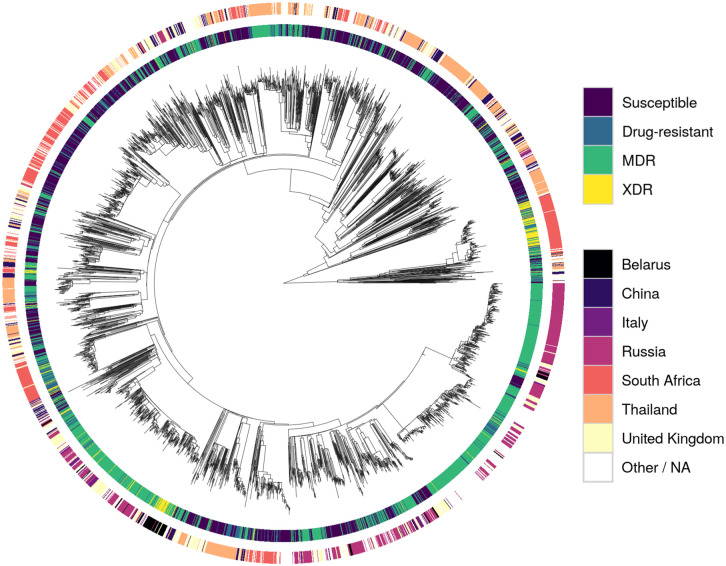
Although the F₁-score was used for ranking models while searching hyperparameter space, the more intuitive recall metric was additionally employed for assessing classifier performance. Calculated for the positive (resistance) and negative (susceptible) case separately, recall is equivalent to the sensitivity or true-positive rate (positive recall) and specificity or true-negative rate (negative recall), respectively. Performance metrics of all models tested are depicted in Fig 3 and listed in Table 3.

Fig 3

Machine learning prediction performance.

F₁-scores (top) as well as negative and positive recalls (bottom; left and right bars of corresponding colour) of all classifiers tested. LR, logistic regression; L1, L1 penalty; L2, L2 penalty; SVM, support vector machine; RBF, radial basis function kernel; DT, decision trees; MD5, maximum depth of five; RF, random forest; GBM, gradient-boosted machines; SDNN, single-drug neural net; MDNN, multidrug neural net.

Table 3

ML prediction performance.

Method	INH			RIF			EMB			PZA			SM			Package	Studies
	F1	R+	R−	F1	R+	R−	F1	R+	R−	F1	R+	R−	F1	R+	R−
Lasso	.95	.92	.98	.96	.94	.99	.78	.77	.89	.76	.77	.88	.93	.90	.97	sklearn	–
LR-L1	.96	.94	.97	.96	.95	.97	.78	.90	.79	.80	.84	.89	.94	.92	.97	sklearn	[21–23, 26]
LR-L2	.95	.93	.97	.95	.93	.97	.78	.89	.80	.76	.84	.84	.94	.92	.96	sklearn	[19, 22–24]
SVM-L1	.96	.94	.98	.96	.94	.98	.79	.90	.82	.79	.81	.88	.94	.91	.97	sklearn	–
SVM-L2	.95	.93	.98	.96	.94	.97	.80	.90	.82	.77	.83	.85	.93	.92	.96	sklearn	[22, 23, 25]
SVM-RBF	.96	.94	.98	.96	.94	.97	.79	.90	.82	.77	.80	.87	.92	.90	.96	sklearn	[20, 22, 23]
DT	.95	.95	.95	.96	.96	.96	.74	.76	.86	.74	.81	.83	.91	.89	.94	sklearn	[26]
DT-MD5	.96	.94	.98	.94	.91	.99	.76	.94	.73	.70	.84	.75	.91	.91	.92	sklearn	[26]
RF	.96	.94	.98	.96	.95	.97	.81	.88	.85	.75	.85	.82	.91	.90	.94	sklearn	[19, 20, 23–25]
GBM	.96	.95	.96	.97	.96	.98	.79	.81	.89	.78	.77	.90	.93	.92	.96	sklearn	[19, 23, 26]
SDNN	.95	.93	.96	.95	.92	.97	.76	.78	.86	.72	.77	.84	.92	.90	.95	Keras	[19, 24]
MDNN	.94	.91	.97	.93	.89	.97	.75	.77	.87	.75	.72	.91	.88	.89	.90	Keras	[24]

Performance metrics of the ML models tested in addition to the underlying Python packages and recent studies employing similar techniques for antibiotic resistance prediction. F₁, F₁-score; R+, positive recall; R−, negative recall; other abbreviations are explained in Fig 3.

For INH, RIF, and SM most models performed similarly well with consistently higher recalls for the ‘susceptible’ class. This observation is not surprising as the resistance of some strains might have been caused by genomic features other than missense-SNPs like indels or SNPs in non-coding regions. Moreover, in some cases, resistance might have been conferred by cooperative networks of SNPs that all need to be present concomitantly in order to take effect. As such networks are likely to be ‘fluctuant’ (i.e. several similar patterns might yield comparable effects) as well as harder to obtain evolutionally (it is more likely to acquire a single or a few strongly selected mutations than a larger number of weakly selected, cooperative ones), they are underrepresented in the dataset and thus not learned effectively. Nonetheless, the recalls are comparable to what was reported in other recent resistance-prediction studies (e.g. [23]) and, for INH and RIF, also to a state-of-the art direct association model [10]. It should be kept in mind, though, that the different studies used different data and hence comparisons should be interpreted carefully.

Surprisingly, for SM all models outperformed the direct association approach [10], even though the rRNA gene rrs was completely absent from the missense-only dataset. However, for EMB and PZA both [23] and [10] outperformed the models tested here with the difference in performance being smaller for PZA. The performance gap between INH, RIF and SM on one hand and EMB and PZA on the other may be partially explained by the latter two datasets being the most imbalanced ones. Additionally, two of the ten most important SNPs for predicting EMB resistance reported by [23] lie outside the coding region of embA and are thus absent from the missense SNPs used here.

Although trained and tested on the same data, there is high variance among the performance metrics of the individual models for the harder-to-predict drugs EMB and PZA. This result could be attributed to stratification within the training/testing splits favouring some models over others. Repeating the fitting and testing process multiple times as done in some other studies [22, 23, 53] might smooth out the variation but was infeasible given the computational resources available for this work.

Remarkably, NNs did not outperform the simpler learning algorithms and the multidrug version did consistently worse than its single-drug counterparts. It should be noted, though, that the space of possible network architectures, regularisation methods, loss functions and optimisers with accompanying hyperparameters is tremendously vast and a proper hyperparameter search for deep NNs was not in the scope of this work. Nonetheless, despite exploring more complex NN architectures, Chen et al. also found that L2 regularised logistic regression performed on a par with their best neural nets [24]. In combination with the results reported here, this might indicate that—given the rather direct relationship between genotype and phenotype—the higher complexity of NNs is not justified. Overall, the results do not show a clear trend towards a single method or family of algorithms and most models performed comparably well.

The 20 most important SNPs of all classifiers allowing for extraction of feature importances are illustrated in Fig 4. Linear SVM and especially Lasso appeared to be less sensitive to co-occurring resistance, whereas all other models seemed to be affected equally with true and false positives occurring at roughly the same rate. Lasso’s greater robustness might be attributed to it being a regression rather than a classification method. Therefore, its output is not bounded between 0 and 1 and the model tries to keep the prediction for resistant strains as close to 1 as possible since overestimating the resistance status would increase the error just as much as underestimating it would. Conversely, all the other methods are implemented as proper classifiers only capable of producing class probabilities between 0 and 1. Thus, taking prediction of INH resistance as an example, giving large weight coefficients to S315 in katG as well as S450 in rpoB, which are both present in ∼1,200 strains, would let Lasso predict a number close to 2 for most samples, whereas logistic regression due to its sigmoid nature would only be even more sure that the sample is 1, i.e. resistant.

Fig 4

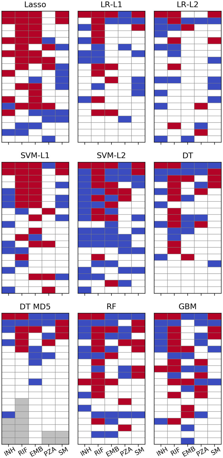
Machine learning feature importance.

Top 20 SNPs per ML algorithm as sorted by the respective measure of feature importance. Cells are coloured red for SNPs in genes known to contribute to resistance to the respective drug and blue for SNPs involved in resistance to other drugs. Grey cells denote a feature importance of zero or a p-value of 1 (i.e. there are fewer than 20 SNPs with non-zero feature importance). p-values for LR have been calculated with approach 1.

However, regression coefficients for strongly correlated genotypes (e.g. compensatory or cooperative mutations) are likely to be underdetermined and hence unstable in Lasso. This would make Ridge regression [ordinary least squares (OLS) with L2 penalty] [54] or Elastic Nets (OLS with linear combination of L1 and L2 penalties) [55] better choices for exploring feature importance in such cases as the quadratic penalty forces coefficients of collinear predictors to take similar values. These methods have not been tested systematically in this work, though.

For PZA not a single algorithm ascribed highest relevance to a SNP in pncA and in L1 regularised logistic regression the most important SNP from that gene appeared only at rank 23. It should be noted, however, that the plots for logistic regression in Fig 4 are based on the p-values calculated with approach 1 (see Methods) which should be viewed only as an easily available heuristic for feature importance. When sorted by absolute magnitude of regression coefficients, six pncA SNPs were featured in the top 20 (see S6 Fig and S4 Data).

The white tiles in Fig 4 represent “unknown” SNPs that have not been linked to resistance so far (we define “unknown” as not being present in the TBProfiler [10] database). They are listed in more detail in S4 Table and some show very favourable p¹ g¹ / p⁰ g¹ ratios. However, upon closer inspection of their distribution across the phylogeny, for most variants the association appears to be due to population stratification. This is also evident from their relatively small average pairwise distance values. A SNP in a hypothetical protein (genome position 2238734), for instance, occurred in 78 samples resistant against RIF and only in seven that were susceptible. Yet, all strains carrying the mutation are located on the same clade in the phylogenetic tree (S7 Fig). Nonetheless, a few promising candidates were found (Table 4). P93 in idsB, for example, appeared in 12 INH-resistant and two susceptible strains and has emerged multiple times independently (S8 Fig). Moreover, nine of the 12 resistant samples also carried a resistance-conferring SNP in katG. Thus, one could argue that idsB P93 might have a compensatory effect reducing the fitness penalty incurred by the katG mutations.

Table 4

Potential novel variants related to resistance extracted from the ML feature importances.

Drug	Gene	Locus Tag	Position	Ref. AA	Codon	p1 g1	p0 g1	Distance	Method	Rank	Comment
INH	idsB	Rv3383c	3798212	P	93	12	2	0.688	SVM-L1	19	possibly compensatory for katG
RIF	.	Rv2348c	2626678	I	101	10	4	1.484	SVM-L1	18	strong homoplasy, but many susceptible strains and overlap with rpoB in resistant strains
	.	Rv3467	3884871	P	303	30	15	1.172	SVM-L2	19
PZA	rpoB	Rv0667	761314	F	503	8	1	0.522	Lasso	16	probably false positive and actually related to RIF overlap with pncA
	.	Rv2670c	2986827	A	5	76	23	0.479	GBM	17

The most promising SNPs with high p¹ g¹ / p⁰ g¹ ratios and large distance values (indicating strong homoplasy) were selected from S4 Table Ref. AA, reference amino acid.

Further, eight samples resistant against PZA featured a mutation in rpoB F503. However, these were all resistant against RIF as well, which—since rpoB is the main target of RIF—might indicate a potential false positive. Nonetheless, rpoB F503 could still represent a novel compensatory variant related to RIF resistance as all strains carrying it also feature rpoB S450.

SNPs at the positions 2626678 and 3884871 (both in hypothetical proteins) showed strong homoplasy, but only two thirds of the strains they appeared in were resistant against RIF. Moreover, all 10 resistant samples with a SNP at 2626678 and 29 out of 30 with a SNP at 3884871 also carried at least one SNP in rpoB. Thus, although perhaps not causing resistance, these variants might provide some other fitness advantage, which has been strongly selected for recently, explaining their frequent independent emergence.

Similarly, position 2986827 (in a hypothetical protein) has also mutated independently multiple times and occurred in 76 strains that were resistant against PZA (vs. 23 susceptible ones). Sixty-one of the resistant samples carried pncA SNPs as well, possibly hinting at a compensatory or cooperative effect. However, the majority of strains featuring a SNP at that position lie within a single clade (S8 Fig). Hence, further research with complementary methods is required to confirm these associations.

Application of Hungry, Hungry SNPos

The last SNPs remaining after 20,000 iterations for every drug as determined by HHS are listed in Table 5. As opposed to most of the other methods, the algorithm re-discovered predominantly true positives. The results in Table 5 were obtained with w_p⁰g¹ = 2, a filter ignoring all SNPs with p¹ g¹ < 5, normalised p¹ g¹ and p⁰ g¹ values, and a distance weight of 1. This set of parameters turned out to be most reliable across the five drugs tested. Additional results are available in S5 Data.

Table 5

’Last SNPos standing’ after 20,000 iterations of HHS.

Drug	Gene	Position	Codon	Ref. AA	p1 g1	p0 g1	Counts	Distance	Score0	Score20000	Resistance
INH	katG	2155541	191	W	10	0	1577.9	1.040	1640.4	237633.6	INH
	katG	2155169	315	S	8	0	1577.9	0.850	1337.1	159553.4	INH
	katG	2155168	315	S	1676	12	1538.7	0.945	1453.4	128838.5	INH
RIF	rpoB	761101	432	Q	10	0	1680.2	1.174	1973.1	135374.4	RIF
	rpoB	761128	441	S	13	0	1680.2	1.032	1733.6	107171.9	RIF
	rpoB	760314	170	V	24	0	1680.2	0.922	1549.1	93596.2	RIF
	rpoB	761139	445	H	135	4	1523.8	1.073	1634.5	74374.8	RIF
	rpoB	761155	450	S	1367	9	1644.6	0.844	1387.9	35940.8	RIF
	rpoB	761110	435	D	131	7	1404.5	1.328	1865.4	30883.7	RIF
EMB	embB	4247495	328	D	7	1	1890.4	1.446	2733.1	57535.3	EMB
	gyrB	6742	501	E	8	1	1960.3	1.217	2385.3	44699.3	FQ
	rpoC	765846	826	N	5	1	1680.8	0.884	1486.6	31274.1	RIF
	embB	4247729	406	G	13	3	1576.0	0.785	1236.5	23067.0	EMB
	rpoB	761097	431	S	5	0	2519.3	0.784	1975.7	22631.1	RIF
	embB	4247469	319	Y	11	3	1441.3	0.852	1228.0	16557.9	EMB
	pncA	2288703	180	V	7	1	1890.4	0.490	926.2	16378.0	PZA
	embB	4248003	497	Q	82	25	1343.9	0.956	1285.2	13938.8	EMB
	embB	4247429	306	M	455	120	1469.4	0.781	1147.5	11245.9	EMB
PZA	pncA	2289096	49	D	6	0	1762.6	0.967	1704.0	31191.7	PZA
	hadA	732110	61	C	5	0	1762.6	1.112	1960.5	27771.6	.
	pncA	2289043	67	S	7	1	1340.8	0.975	1307.3	15491.8	PZA
	pncA	2288839	135	T	9	0	1762.6	1.117	1968.2	13797.6	PZA
	pncA	2289222	7	V	6	2	919.0	0.700	643.5	13649.0	PZA
	pncA	2288820	141	Q	9	1	1425.2	0.655	934.1	11959.5	PZA
	rpoC	766488	1040	P	10	3	983.9	0.778	765.9	8919.5	RIF
	pncA	2289213	10	Q	48	3	1564.1	0.413	646.1	4897.7	PZA
	pncA	2288703	180	V	6	0	1762.6	0.373	657.8	4765.2	PZA
	pncA	2289016	76	T	5	2	798.5	0.855	682.6	4445.3	PZA
	pncA	2289054	63	D	6	1	1280.6	0.376	481.7	2899.9	PZA
	pncA	2289040	68	W	17	1	1575.1	0.598	942.5	1869.5	PZA
	rpoA	3878416	31	G	5	1	1200.2	0.083	99.2	253.2	.
SM	rpsL	781822	88	K	60	7	613.7	0.881	540.4	40005.3	SM
	rpsL	781687	43	K	469	11	791.2	0.632	499.9	22640.5	SM

The algorithm was run with the set of parameters that generalised best across all drugs. ‘Counts’ denotes the intermediary result of the expression in brackets in Eq 1, which is subsequently multiplied by the distance to give the initial score. In this setting, the values for p¹ g¹ and p⁰ g¹ were normalised before being used in the calculations (for details see S3 Methods). SNPs from genes known to be involved in resistance to the respective drug are shaded red. SNPs from genes known to be involved in resistance to other drugs are shaded blue. Ref. AA, reference amino acid.

While runs without the p¹ g¹ filter and w_p⁰g¹ = 10 returned additional relevant low-frequency SNPs for INH, RIF, and PZA, they failed to produce any relevant SNPs for EMB and SM. This is a general risk of running HHS without a filter for rare alleles and normalised p¹ g¹ values since—given equal distance values—SNPs with p¹ g¹ = 2 and p⁰ g¹ = 0 are assigned the same score as SNPs with p¹ g¹ = 1000 and p⁰ g¹ = 0. Additionally, very-low-frequency SNPs are less likely to sufficiently overlap with other strong SNPs which lets them take out truly resistance-conferring variants easily.

Not normalising p¹ g¹ strongly favoured the most common alleles leading to a drastically reduced set of final SNPs (often only one). This is due to high-frequency co-resistant false positives not being removed quickly enough and outliving less common true positives. Setting w_p⁰g¹ to 10 partially mitigated this issue as the initial scores of false positives with non-zero p⁰ g¹ values were substantially lower or negative.

Not accounting for intra-p¹ g¹ distance (i.e. setting the weight for d_{p¹g¹, i} to 0) had substantial influence on the results in most but not all settings. This shows that even a primitive distance metric like the average pairwise Hamming distance is a good surrogate for incorporating population structure.

An exemplary depiction of the changing scores over the course of an HHS run (with the settings used to generate the results in Table 5) is shown in Fig 5. After an initial rise, scores of co-resistant SNPs (blue) slowly decreased until they dropped below zero and the corresponding variants were purged. However, some pncA variants, which almost completely overlapped with the most common co-occurring resistance markers (e.g. katG S315 or rpoB S450), shared the same fate as those did not disappear quickly enough. After increasing the penalty for p⁰ g¹ by setting w_p⁰g¹ to a larger value, co-occurring SNPs started off with lower initial scores and more pncA variants were retained (S5 Data). Additionally, two rare pncA variants (T100 and T160; occurring in eight and nine samples, respectively) overlapped in eight samples and were therefore eliminated quickly.

Fig 5

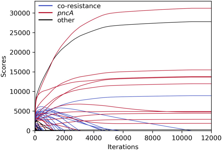
Course of HHS scores for PZA during iterative elimination.

Scores remained unchanged after ∼11,000 iterations. SNPs related to PZA resistance in red; SNPs related to other drugs in blue; other SNPs in black.

All SNPs shaded red or blue in Table 5 are already known to confer resistance to the respective or a different drug. For PZA, however, two variants might constitute novel discoveries and thus warrant closer examination. The rpoA G31 mutation started and finished with an exceptionally low score due to the samples featuring this variant being closely related (resulting in a very low average pairwise distance, S9 Fig). Additionally, it was only found in two out of the 14 different parameter configurations tested (S5 Data). Furthermore, it overlapped with two pncA SNPs (D8 and C138—both are marked as conferring resistance against PZA in the TBProfiler database [10]), which occurred in fewer than five samples and thus were excluded from the dataset. In light of this complementary evidence, it is reasonable to suspect rpoA G31 to be a false positive caused by population structure.

The five strains harbouring hadA C61, on the other hand, were more widely spread out across the phylogeny and the mutation has apparently emerged independently four times (S9 Fig). Moreover, it was among the final SNPs in nine out of 14 HHS runs with different parameters. However, three of the five samples carrying hadA C61 also featured pncA variants that confer resistance according to TBProfiler (T100, V139, V180). Two of these were too rare to be included in the analysis and for the third one the initial score was already below 0. Therefore, hadA C61 might likewise be a spurious result and its validity should be checked by including more samples or consulting orthogonal methods in future work.