1 INTRODUCTION

Carbon (C) fixation via photosynthesis is known as gross primary production (GPP) when assessed at the ecosystem level, and together with ecosystem respiration it dominates the land‐atmosphere exchange of carbon dioxide (CO₂) (Ryu et al., 2019). GPP is thus one of the main processes driving climate regulation, C sequestration and C storage (Le Quéré et al., 2018) as well as being an important proxy for a range of ecosystem services, including the production of food, fibre and fuel, and the regulation of the habitability of Earth (Rockström et al., 2009; Steffen et al., 2015). Human population growth and increased food and fibre consumption have increased the use of global primary production (Krausmann et al., 2017), with severe consequences for services and functions of global ecosystems (Rockström et al., 2009; Steffen et al., 2015). An improved understanding of spatial and temporal dynamics in regional and global GPP is additionally essential to better understand, quantify and forecast the effects of current and future climate change (Tagesson et al., 2020), also in relation to design of climate change mitigation policies and in the early detection of ecosystem change (IPBES, 2018).

Models driven by satellite‐based Earth observation data are commonly used for quantifying GPP for large areas, allowing to evaluate the role of GPP within the global carbon cycle (Ciais et al., 2013). The most common approach for estimating GPP from satellite data involves the light use efficiency (LUE) model, where LUE is defined as the conversion efficiency of absorbed photosynthetically active radiation (PAR) into GPP (Madani et al., 2014; Monteith, 1972, 1977; Potter et al., 1993; Ruimy et al., 1994; Running et al., 2004). The LUE concept has been applied in various methods, either by using a biome‐specific LUE (Ruimy et al., 1994) modified using meteorological variables (Running et al., 2004), or modified using plant traits (Madani et al., 2014). The LUE model can be formulated as the product of incoming radiation, the fraction of PAR absorbed by the vegetation (FAPAR), and the LUE; where LUE and PAR provide the relationship between GPP and light, whereas FAPAR incorporates dynamics in green vegetation cover.

The advantage of the LUE model is its simplicity using a linear relationship, and it has been shown to work well in a range of biomes and environmental conditions (Kolby Smith et al., 2015; Martínez et al., 2020; Running et al., 2004; Ryu et al., 2019; Stocker et al., 2019; Tagesson, Mastepanov, et al., 2012). However, this simplicity also comes with a cost. For the assumption of a linear relationship to be valid, the intercept between GPP and absorbed PAR must equal zero, as otherwise a systematic error is introduced. Observations show that the relationship between GPP and PAR generally follows an asymptotic shape, and only by multiplying with FAPAR does the relationship turn approximately linear (Baldocchi, 1994; Falge et al., 2001; Lindroth et al., 2007; Monteith, 1972; Ruimy et al., 1995; Tagesson, Fensholt, Cropley, et al., 2015). However, when FAPAR approaches one, this linearization does not occur, and the actual relationship thereby remains asymptotic. Furthermore, the LUE‐derived GPP strongly depends on FAPAR, as it sets the maximum level of absorbed PAR, and thereby also the maximum level of GPP during a certain phenological phase. FAPAR is generally defined as PAR absorbed by green vegetation, but there is yet no exact definition of ‘green’ in this context. In reality, PAR is strongly absorbed by all components of the canopy, and an estimate of ‘green FAPAR’ is therefore impossible to verify based on ecosystem‐scale field observations. Finally, there is a hysteresis in the GPP‐absorbed PAR relationship, since LUE is not the same during different phases of the phenological cycle (Madani et al., 2014; Ryu et al., 2019; Tagesson, Fensholt, Cropley, et al., 2015).

Global‐scale Earth observation‐based GPP products are of high societal relevance, and current products are based either on LUE, or machine learning techniques (Booth et al., 2012; Jung et al., 2011; Kolby Smith et al., 2015; Running et al., 2004; Stocker et al., 2019; Yao Zhang et al., 2017). To better accommodate for the nonlinear relationship known to exist between PAR and carbon assimilation, we take an ecosystem‐level physiologically realistic approach by instead converting Earth observations to biome‐specific parameters of an asymptotic relationship between GPP and PAR, referred to as the light response function (LRF). We further analyse the impact of local air temperature (T _air), soil water content (SWC), vapour pressure deficit (VPD) and atmospheric CO₂ concentrations on GPP, and test relevant relationships to constrain LRF‐modelled GPP. We then apply these relationships biome‐wise to derive spatially explicit estimates of GPP globally. The new GPP estimates derived using the LRF model are cross‐validated against ground observations and compared to a set of state‐of‐the‐art Earth observation GPP products. Finally, the LRF‐based GPP product is used for quantifying dynamics in global‐scale GPP budgets over the period 1982–2015 and the contribution from different terrestrial regions to the global GPP.

2 MATERIALS AND METHODS

2.1 Data collection and pre‐processing

2.1.1 Gridded data

NDVI and land cover data

The Global Inventory Monitoring and Modelling System third generation (GIMMS3g) data archive is based on observations by the advanced very high resolution radiometer (AVHRR) (Pinzon & Tucker, 2014). GIMMS3g provides global semi‐monthly normalized difference vegetation index (NDVI) at 1/12° spatial resolution for the period 1981 to 2015. Among all existing long‐term AVHRR‐based datasets, the GIMMS3g NDVI time series has been shown to have the highest temporal consistency, decreasing the risk of artefacts caused by sensor shifts (Tian et al., 2015).

The MCD12C1 version 6 land cover type product (land cover as defined by the International Geosphere Biosphere Programme, IGBP) is derived from Moderate Resolution Imaging Spectroradiometer (MODIS) observations based on a combined dataset of Terra and Aqua platforms. It provides the dominant land cover type at a spatial resolution of 0.05° × 0.05°. No global dynamic IGBP dataset exists for the full period 1982–2015, and we therefore used the MCD12Q1 product for 2001 (representing the middle of our study period). The multiple IGBP classes were simplified to eight ‘biomes’ by merging the following land cover classes: closed shrublands (IGBP class 6), open shrublands (7) and woody savannahs (8) were merged with the class savannahs (9). Permanent wetlands (11) were merged with grasslands (10). The cropland/natural vegetation mosaic class (14) was combined with croplands (12). Urban (13), snow and ice (15), and barren or sparsely vegetated (16) were combined. The final biomes recognised were evergreen needleleaf forest; evergreen broadleaf forest; deciduous needleleaf forest; deciduous broadleaf forest; mixed forest; savannah/shrublands; grasslands; and croplands.

Ancillary meteorological data

We downloaded daily European Centre for Medium‐Range Weather Forecasts (ECMWF) Reanalysis (ERA)‐interim T _air at 2 m height (in degrees K), volumetric soil water in 0–0.07 m soil depth (m³ m^‐3), downwelling shortwave solar radiation at the surface (W/m²), and total column water vapour (kg/m²) from 1982 to 2015. Data had a spatial resolution of 0.25° × 0.25°, and were available for every 12 hr period (daytime and night‐time) (Dee et al., 2011; ECMWF, 2016), which were averaged to daily values. PAR (W/m²) was estimated as 46% of the downwelling shortwave radiation (Iqbal, 1983).

All gridded data were resampled to 0.05° × 0.05° resolution using bilinear interpolation to be collocated and having identical spatial resolutions.

Global‐scale GPP and solar‐induced fluorescence products

In order to compare our modelled GPP against previous GPP products, we included six state‐of‐the‐art GPP products based on Earth observation data (Table 1). Based on data from MODIS, we used: the MOD17GPP collection 5.5 (Running et al., 2004), the Soil Moisture Active Passive (SMAP) GPP product (Booth et al., 2012) and the Vegetation Photosynthesis Model (VPM) GPP product (Zhang et al., 2017). Based on GIMMS3g NDVI we used: GPP as modelled by the P‐model (Stocker et al., 2019), GPP from FLUXCOM (Jung et al., 2011) and GPP modelled with a MOD17‐based algorithm by Kolby Smith et al. (2015).

Table 1

Overview of global‐scale gross primary production (GPP) and Solar‐Induced Fluorescence (SIF) products. The products of GPP are: light response function (LRF)‐modelled GPP developed in this study, GPP from FLUXCOM, Kolby Smith‐modelled GPP using the MOD17‐based algorithm, GPP as modelled by the P‐model, the MOD17GPP, the Soil Moisture Active Passive (SMAP) GPP and the Vegetation Photosynthesis Model (VPM) GPP. For SIF, we used the contiguous SIF (CSIF) dataset. Information of spatial and temporal resolution, study period of the products and their references are included

Product	Spatial resolution	Temporal resolution	Study period	Reference
LRF	0.05° × 0.05	Daily	1982–2015	(This study)
FLUXCOM	0.5° × 0.5	Monthly	1982–2015	Jung et al. (2011)
Kolby Smith	0.5° × 0.5	Monthly	1982–2015	Kolby Smith et al., (2015)
P‐model	0.5° × 0.5	Daily	1980–2013	Stocker et al., (2019)
MOD17	0.5° × 0.5	Monthly	2000–2016	Running et al., (2004)
SMAP	9 × 9 km2	Daily	2000–2016	Booth et al., (2012)
VPM	0.05° × 0.05	8‐day	2000–2016	Zhang et al., (2017)
CSIF	0.05° × 0.05	4‐day	2000–2017	Zhang et al., (2018)

Solar‐induced fluorescence (SIF) is light emitted during photosynthesis, and thereby supposedly a proxy for GPP (Zhang et al., 2018). We used a contiguous global coverage product (CSIF), developed from Orbiting Carbon Observatory‐2 (OCO2) SIF data by training a neural network using MODIS surface reflectance data (Zhang et al., 2018). Dynamics in CSIF are consistent with SIF from OCO‐2 and the Global Ozone Monitoring Experiment‐2 (GOME‐2), but have a longer time series and the same spatial resolution as used in this study (Table 1).

2.1.2 Site data

Eddy covariance data and atmospheric CO₂ concentrations

Daily GPP observations (partitioned with the daytime methods, with variable user threshold, i.e. the variable called GPP_DT_VUT_MEAN) were acquired from the Tier 1 and Tier 2 database of FLUXNET 2015 (Pastorello et al., 2020). FLUXNET is a global network of micrometeorological flux measurement sites measuring net CO₂ exchange using the eddy covariance method. FLUXNET2015 collated measurements from 212 of these sites into an open database. To ensure an accurate point‐to‐pixel comparison, only sites measuring fluxes over the same land cover as the dominant cover of the associated MCD12C1 pixels were included. Additionally, ten sites located close to confounding elements for NDVI, such as rivers, oceans or towns were disregarded. In this study, 79 of the 212 sites were used (Table S1). From the selected sites, only GPP with high‐quality control flags (>0.5) was used in the final analysis.

Atmospheric CO₂ concentrations derived from in situ air measurements at Mauna Loa, Hawaii were retrieved from the NOAA Earth System Research Laboratories (ESRL) (Keeling et al., 2005).

NPP data

To further evaluate the modelled GPP data against an independent ground observation dataset, we downloaded the net primary productivity (NPP) estimates compiled by the Global Primary Production Data Initiative (GPPDI) (Olson et al., 2013). From the GPPDI version B dataset, we extracted NPP from all sites which had an uncertainty flag value lower than 50. In total, it was 157 site‐years distributed globally across 58 sites between 1982 and 1998 (Olson et al., 2013).

2.3 Relationships with explanatory variables

For an overview of the workflow of the model development, see Figure 1.

Figure 1

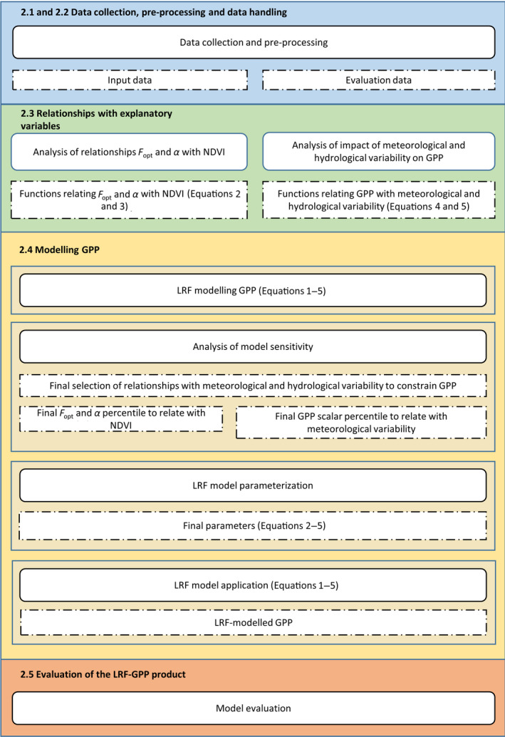
Overview of the workflow of the model development and evaluation. Rectangles with rounded corners present methods whereas rectangles with dashed borders are output of these. Coherent steps of the workflow are colour‐coded, and referred to by their respective subheadings. F _opt is the optimized carbon uptake at light saturation (photosynthetic capacity; g C m⁻² day⁻¹), and α is the quantum efficiency (g C W^‐1 PAR)

2.3.1 Coupling photosynthetic capacity and quantum efficiency with NDVI

In order to spatially and temporally extrapolate GPP; we parameterized logistic relationships between the parameters of the LRF model (F _opt and α in Equation 1) and GIMMS3g NDVI for each biome:

$F_{\text{opt}}=\frac{F_{\text{optmax}}}{1‐\exp (b_{F_{\text{opt}}}\times \text{NDVI}+F_{\text{optmid}})},$ (2)

$\alpha =\frac{{\alpha }_{tmax}}{1‐\exp (b_{\alpha }\times \text{NDVI}+{\alpha }_{\text{mid}})},$ (3)

where F _optmax and α _max are the maximum possible F _opt and α for the specific land cover class, F _optmid and α _mid are parameters of the logistic functions denoting the NDVI midpoint of the function, and b _fopt and b_α represent the steepness of the curve. A logistic function was chosen as it turned out to describe the response of F _opt and α to NDVI well (Section 3.1).

In the first estimates of F _opt and α (Section 2.2.2 above), a large fraction of the variability was caused by spatial and temporal variability in biogeophysical conditions. Therefore, in a model optimization procedure, we used biome‐specific percentiles of F _opt and α for 20 equally sized NDVI bins when fitting the functions. We fitted all F _opt and α percentiles (1–100) and modelled GPP for each F _opt and α percentile combination (Section 2.4.2 below). The final biome‐specific percentile used was the one generating the lowest root‐mean‐square‐error (RMSE) in the subsequent model evaluation (Figure 2; Table 2).

2.3.2 Impact of meteorological and hydrological variability on GPP

In order to derive relationships used for constraining GPP within the modelling framework (Figure 1), we analysed impacts of daily variability in meteorological and hydrological conditions (T_air, CO₂, SWC and VPD) on daily GPP. We clustered the daily FLUXNET2015 GPP by separating the meteorological and hydrological data into bins (bin width: T_air: 5°C; SWC 5%Vol; CO₂ 5 ppm; VPD 25 hPa) and extracted the 50th and 98th percentile GPP associated with each bin. The 50th percentile indicates the median impact of the meteorological and hydrological variables, whereas the 98th percentile indicates the upper boundary for GPP.

A large fraction of the GPP variability caused by meteorological and hydrological variability is already captured by the NDVI variability, and is therefore already included in the GPP modelled by Equations (1), (2), (3). In order to estimate GPP that is not captured by Equations (1), (2), (3), we calculated a GPP scalar by taking the ratio of measured GPP and GPP modelled using Equations (1), (2), (3). This is considered to be GPP variability caused by short‐term meteorological and hydrological variability, whereas Equations (1), (2), (3) capture seasonal dynamics in GPP caused by phenological drivers. We first used regression tree analysis to determine the variable importance of the meteorological and hydrological variables (Supplementary subsection S2). The environmental variables were introduced in the GPP model in the order of the variable importance for the different biomes. We thereafter analysed impact of daily variability in meteorological and hydrological conditions (T _air, CO₂, SWC and VPD) on the GPP scalars. These GPP scalars were also separated using the meteorological and hydrological bins described above and the 50th and 98th GPP scalar percentiles were extracted from each bin.

The relationships between the GPP and T _air, and GPP and VPD turned out to follow logistic curves (Section 3.1; Supplementary subsection S3). We therefore fitted such a function with 50th and 98th percentile binned GPP, and 50th and 98th percentile GPP scalar for each biome:

$f(\text{ENV})=\frac{a_{\text{max}}}{1‐\exp (k\times \text{ENV}+b_{\text{mid}})},$ (4)

where f(ENV) is a function for constraining GPP due to variability in the meteorological variables (ENV; in this case T _air, and VPD). a _max, k and b _mid are parameters of the logistic function giving the maximum value of the function, steepness of the curve and the ENV value at the midpoint of the function respectively.

The relationship between GPP and SWC turned out to follow a bell‐shaped curve, and we thereby fitted a Gaussian function as it turned out to describe the response with 50th and 98th percentile binned GPP, and 50th and 98th percentile GPP scalar well (Section 3.1; Supplementary Subsection S3):

$f(\text{SWC})=a_{\text{max}}\times \exp \frac{{(‐\text{SWC}‐b_{\text{mid}})}^2}{2\times b_{\sigma }},$ (5)

where f(SWC) is a function to constrain GPP variability due to SWC stress. a _max, b _mid and b_σ are parameters of the Gaussian function giving the peak value of the curve, the position at the centre of the peak, and the width of the curve (i.e. the standard deviation of the response of GPP to a change in SWC) respectively.

3 RESULTS

3.1 Relationships with explanatory variables

3.1.1 Photosynthetic capacity and quantum efficiency in relation to NDVI

The relationships between F _opt and α and NDVI are highly variable and we therefore extracted percentiles of F _opt and α for NDVI bins before studying the relationships (Figure 2). Strong logistic relationships then emerged between binned F _opt and α and NDVI for all biomes (Figure 2; Table S3). Only few estimates of α were available for the deciduous needleleaf and deciduous broadleaf biomes, and the fitted relationships generated unrealistically large α values when NDVI was high. Maximum binned α were therefore used as a limit (Figure 2).

Figure 2

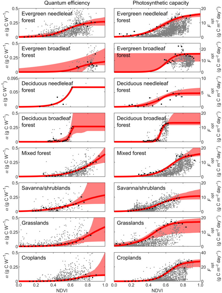
Relationship between quantum efficiency (α) and photosynthetic capacity (F _opt) and the normalized difference vegetation index (NDVI). Shown are: all data (grey dots), percentiles of GPP extracted from NDVI bins (biome‐wise percentiles given in Table 2; black dots), and the fitted logistic relationships (red lines) including the 5^th to 95^th confidence interval obtained from bootstrapping (shaded area)

The sensitivity test indicated that LRF‐GPP is substantially more sensitive to variation in F _opt than α (Figure 3; Supplementary Subsection S5). The sensitivity was also larger at lower F _opt and α percentiles, as the upper percentiles GPP are instead constrained by the environmental scalars. From this sensitivity space, the F _opt and α percentiles generating the lowest RMSE can be extracted, and these percentiles were used in the final model parameterization.

Figure 3

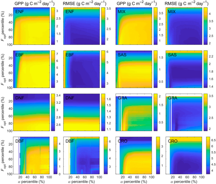
Sensitivity of modelled gross primary production (GPP) to variability in optimized carbon uptake at light saturation (F _opt) and quantum efficiency (α). Shown is the impact on GPP and the root‐mean‐square‐error (RMSE) for: evergreen needleleaf forest (ENF); evergreen broadleaf forest (EBF); deciduous needleleaf forest (DNF); deciduous broadleaf forest (DBF); mixed forest (MIX); savannah/shrublands (SAS); grasslands (GRA); and croplands (CRO). White areas are caused by too few data in the bins. Note that scales differ for the different biomes. For coefficient of determination (R ²) and slope and intercept from ordinary least square linear regression fitted between modelled and field measured GPP, see Supplementary Subsection S5

3.1.2 Impact of meteorological and hydrological variability on GPP

Strong relationships between median binned GPP, and T _air, VPD and SWC exist (Figure 4; Supplementary Subsection S2–S3). Generally, most of the variability was explained by one dominant factor and the remaining variables explained substantially less (Table S2). After NDVI and PAR, T _air was the dominant constraining variable explaining GPP variability in most biomes (Figure 4; Supplementary Subsection S2–S3). For all biomes except savannah/shrublands and grasslands, upper boundaries of GPP were also found against T _air (Figure 4; Supplementary Subsection S4). The second most important variable was SWC, where upper boundaries of GPP were observed for all biomes except for evergreen broadleaf forest and croplands (Figure 4; Supplementary Subsection S3). The optimal SWC level was quite similar among biomes, ranging between 26% and 31% (Table S5). The widest range in the response of GPP to SWC was found for mixed forest (Figure 4; Table S5, as indicated by the standard deviation of the fitted Gaussian curve). Finally, VPD was found to constrain GPP in savannah/shrublands and grasslands, with associated upper GPP boundaries (Figure 4).

Figure 4

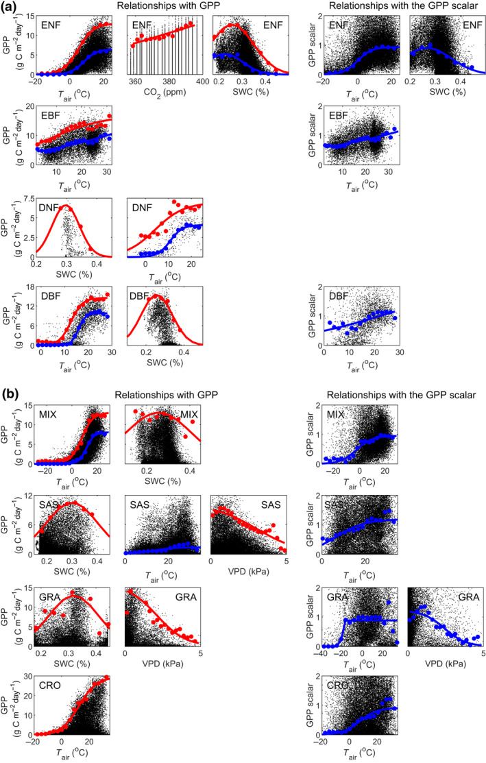
Relationships between gross primary production (GPP) and the constraining environmental variables: air temperature (T _air), soil water content (SWC), atmospheric carbon dioxide (CO₂) concentrations and vapour pressure deficit (VPD). Shown are relationships for (a) the biomes: evergreen needleleaf forest (ENF); evergreen broadleaf forest (EBF); deciduous needleleaf forest (DNF); deciduous broadleaf forest (DBF); and (b) the biomes: mixed forest (MIX); savannah/shrublands (SAS); grasslands (GRA); and croplands (CRO). Only those constraining variables with strong relationships against median GPP (blue), upper GPP boundary (98th percentile; red) and against the median GPP scalars are included. For all relationships, see Supplementary Information Subsection S3

After GPP had been modelled with the light response functions (Equations (1), (2), (3)), which accounted for the variation associated with NDVI and PAR, GPP variability caused by T _air was still not fully captured for any biome except for deciduous needleleaf forest (Figure 4; subplots against GPP scalars; supplementary subsection S3). The GPP variability caused by SWC and VPD was neither well captured by Equations (1), (2), (3) for evergreen needleleaf forest and grasslands respectively (Figure 4).

The sensitivity analysis for LRF‐GPP against variability in the T _air, SWC and VPD scalars indicated that the percentiles generating the lowest RMSE value were relatively close to the median values (Figure 5). At the lower and higher percentiles, RMSE values were substantially larger (Figure 5). From this sensitivity test, the T _air, SWC and VPD scalar percentiles generating the lowest RMSE were extracted, and these percentiles were used in the final model parameterization. The SWC and VPD scalars did not further reduce the lowest RMSE for evergreen needleleaf forest and grasslands respectively (Figure 5). These scalars were therefore excluded from the final model. The upper boundary of CO₂ for evergreen needleleaf forest (Figure S1), decreased the model performance (data not shown) and was therefore also excluded.

Figure 5

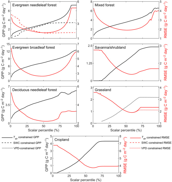
Sensitivity of the gross primary production (GPP) model to variability in environmental scalars (air temperature (T _air), soil water content (SWC) and vapour pressure deficit (VPD)). The T _air scalars were applied for all biomes except for deciduous needleleaf forest. For evergreen needleleaf forest and grasslands, a SWC and a VPD scalar were additionally applied respectively. Note that scales differ for the different biomes. The percentiles of each scalar were extracted and the constraining models were fitted. Shown is the impact of this percentile fitting on GPP (black), and root‐mean‐square‐error (RMSE) (red). For remaining statistics, see Supplementary Information Subsection S5.2

3.2 Model evaluation

The model evaluation indicates that the LRF‐GPP captured the variability in field observations relatively well for all biomes except evergreen broadleaf forest (Table 2), where the average GPP was still well captured but the variability was underestimated (as indicated by slope and intercept in Table 2; Figure S24).

Table 2

Statistics for the bootstrap simulations of gross primary production (GPP; g C m⁻² day⁻¹) and percentiles generating the lowest root‐mean‐square‐errors (RMSE). The uncertainty is ±1 standard deviation from the bootstrap simulations. The numbers in parentheses are the International Geosphere Biosphere Programme (IGBP) land cover classes. F _opt is the optimized carbon uptake at light saturation (photosynthetic capacity; g C m⁻² day⁻¹), α is the quantum efficiency (g C W⁻¹ PAR), T _air is air temperature, and R ² is the coefficient of determination

Biome	F opt percentile	α percentile	T air percentile	Mean GPP	Bias	RMSE	Slope	intercept	R 2
Evergreen Needleleaf Forest (1)	98	76	53	3.2 ± 0.6	−0.00 ± 0.59	1.40 ± 0.19	0.67 ± 0.14	1.10 ± 0.42	0.65 ± 0.09
Evergreen Broadleaf Forest (2)	97	50	50	7.0 ± 1.4	0.10 ± 1.81	1.56 ± 0.58	0.27 ± 0.21	5.18 ± 1.67	0.20 ± 0.15
Deciduous Needleleaf forest (3)	17	50		2.8 ± 0.14	−0.03 ± 0.14	1.16 ± 0.04	0.78 ± 0.04	0.63 ± 0.04	0.61 ± 0.01
Deciduous broadleaf forest (4)	72	76	54	5.9 ± 0.4	−0.30 ± 0.48	2.15 ± 0.39	0.93 ± 0.12	1.21 ± 0.55	0.83 ± 0.07
Mixed forest (5)	97	74	52	3.4 ± 0.71	0.13 ± 1.01	1.52 ± 0.46	0.74 ± 0.25	0.86 ± 0.30	0.72 ± 0.14
Savannah/shrublands (6–9)	61	50	58	1.5 ± 0.55	0.23 ± 0.43	0.88 ± 0.24	0.47 ± 0.15	0.67 ± 0.41	0.52 ± 0.17
Grasslands (10,11)	94	29	57	1.4 ± 0.46	0.28 ± 0.64	1.42 ± 0. 45	0.63 ± 0.23	0.40 ± 0.27	0.48 ± 0.15
Croplands (12)	85	42	61	2.5 ± 0.86	1.08 ± 0.90	2.15 ± 0.80	0.40 ± 0.14	1.06 ± 0.58	0.51 ± 0.17

The evaluation of seven global Earth observation GPP products (including the LRF‐GPP developed in this study) showed that all products captured variability of the FLUXNET2015 GPP well (Figure 6; Table 3; Table S6). Firstly, on global scale, they captured variability well when GPP was averaged across sites, averaged annually and by day‐of‐year (Figure 6; Table 3). The LRF‐GPP captured spatial variability best, SMAP and VPM captured seasonal dynamics best (as given by day‐of‐year average), whereas inter‐annual dynamics were overall best captured by the MOD17 (Figure 6; Table 3; Table S6). Some hysteresis is visible in most of the GPP products (day‐of‐year averages forming circles in Figure 6). Secondly, when separated into biomes, all GPP products captured the variability represented by the FLUXNET2015 GPP well (Table S6). The LRF‐GPP then captured variability better or at least equally well as the other GPP products (Table S6; slope closer to 1.0, and lower RMSE and bias). LRF‐GPP captured the seasonal dynamics well on a global‐scale average (Figure 6), but also agreed well with the seasonal dynamics for the different biomes (Figure S25). The seasonal dynamics were better captured than by the other GIMMS3g NDVI‐based GPP products, and equally well as the MODIS‐based GPP products (Figures S25–S31).

Figure 6

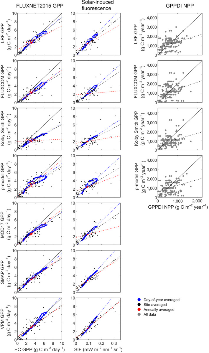
Evaluation of the Earth observation‐based products of gross primary production (GPP). Included comparisons are: eddy covariance (EC)‐based GPP from the 79 FLUXNET2015 sites used in this study; solar‐induced fluorescence (SIF) extracted from the 79 FLUXNET2015 sites; and annual sums of GPP against annual sums of net primary production (NPP) of the Global Primary Production Data Initiative (GPPDI) sites. A one‐to‐one line is included in the FLUXNET2015 comparison whereas in the GPPDI comparison a two‐to‐one line is included since the NPP/GPP ratio is ~0.5 (Landsberg et al., 2020). For statistics of the linear relationships, see Table 3

Table 3

Statistics for the linear regression analysis comparison between Earth observation‐based and eddy covariance (EC)‐based gross primary production (GPP; g C m⁻² day⁻¹), and Earth observation‐based GPP against solar‐induced fluorescence (SIF; mW m⁻² nm⁻² sr⁻¹) extracted from the FLUXNET2015 sites. RMSE is the root‐mean‐square‐error and R ² is the coefficient of determination

Models		EC GPP			SIF
	RMSE	Slope	Intercept	R 2	Slope	Intercept	R 2
LRF‐GPP
Spatial	0.02	0.85	0.44	0.82	25.0	0.4	.79
Inter‐annual	0.02	0.56	1.35	0.42	17.7	1.1	.48
Intra‐annual	0.15	0.89	0.19	0.96	32.0	0.2	.97
FLUXCOM
Spatial	0.62	0.68	0.27	0.63	21.1	0.2	.69
Inter‐annual	0.62	0.78	−0.06	0.71	2.6	1.9	.04
Intra‐annual	0.81	0.80	−0.19	0.97	27.2	−0.4	.97
K Smith
Spatial	0.78	0.55	0.52	0.56	16.2	0.4	.56
Inter‐annual	0.78	0.05	2.03	0.01	5.0	1.6	.01
Intra‐annual	1.02	0.62	0.17	0.97	20.2	0.2	.99
P‐model
Spatial	0.13	0.65	0.85	0.60	18.2	0.9	.59
Inter‐annual	0.26	0.87	0.26	0.59	11.2	1.5	.24
Intra‐annual	0.13	0.76	0.50	0.85	27.8	−0.0	.88
MOD17
Spatial	0.25	0.72	0.54	0.72	20.7	0.5	.74
Inter‐annual	0.25	0.84	0.02	0.55	7.8	1.8	.13
Intra‐annual	0.50	0.76	0.26	0.96	29.4	−0.2	.98
SMAP
Spatial	0.08	0.73	0.86	0.75	22.8	0.7	.87
Inter‐annual	0.08	0.78	0.64	0.81	20.9	0.9	.62
Intra‐annual	0.05	0.90	0.27	0.98	32.9	−0.2	.99
VPM
Spatial	0.05	0.77	0.60	0.69	26.0	0.3	.90
Inter‐annual	0.05	0.75	0.66	0.79	25.4	0.4	.73
Intra‐annual	0.14	1.07	−0.36	0.99	38.0	−0.8	.99

In the comparison against SIF data, all products captured both global‐scale spatial, inter‐ and intra‐annual variability well (Figure 6; Table 3). SMAP and VPM captured SIF‐variability better than the GIMMS3g NDVI‐based models (including LRF‐GPP). All products captured the seasonal dynamics in global‐scale average SIF well (Figure 6), and they also agreed well on the seasonal dynamics for the different biomes (Figures S32–S38).

Finally, the variability in GPPDI NPP was relatively well captured by the GIMMS3g NDVI‐based GPP models, even though they underestimated high and overestimated low NPP (Figure 6; Table S7). When assuming that NPP is about half of GPP (Landsberg et al., 2020), the GPP levels were on average fitted well, especially by the LRF‐GPP and the FLUXCOM GPP models (Table S7). Most data points are located close to the 2 to 1 line, indicating that the GPP products agree well with the variability of NPP (Figure 6).

3.3 Global patterns revealed by LRF‐GPP

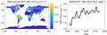
The LRF‐GPP quantifies an annual average global terrestrial GPP budget of 121.8 ± 3.5 Pg C (±1 standard deviation of inter‐annual variability) for the period 1982–2015. High values were found in the areas of tropical evergreen broadleaf forest, whereas arid regions and high northern latitudes have lower average GPP (Figure 7a). The latitudinal distribution of average GPP shows higher values around the equator and a poleward decrease, with a strong drop around 15° North, corresponding to the subtropical deserts.

Figure 7

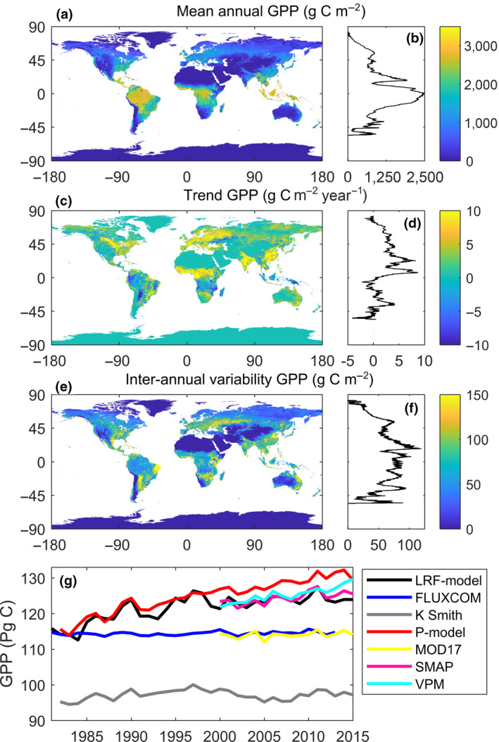
Patterns in light response function (LRF) modelled gross primary production (LRF‐GPP) 1982–2015. (a) Spatial distribution of mean GPP; (b) latitudinal distribution in mean GPP; (c) spatial distribution of trends in GPP 1982–2015; (d) latitudinal distribution in trends in GPP; (e) spatial distribution of inter‐annual variability in de‐trended GPP; (f) latitudinal distribution in inter‐annual variability in de‐trended GPP; and g) a time series 1982–2015 of global‐scale budgets of GPP for the different Earth observation‐based GPP products (see Table 1 for overview of products)

With the new LRF‐GPP product, a pronounced trend in global‐scale terrestrial GPP was observed with an increase of 0.27 ± 0.02 Pg C year⁻¹ (±1 standard error of fitted slope) for the period 1982–2015 (Figure 7g). The latitudinal distribution of the trends is different to the latitudinal distribution of mean GPP, and the trends are generally larger in the northern compared to the southern hemisphere (Figure 7d). The regions with the largest positive trends were located in India, China, Eastern Europe and West Africa (Figure 7c). These regions have substantial areas with croplands, and West Africa recovered from a strong multi‐decadal drought during this period. Large parts of the tropics, especially Papua New Guinea, Indonesia, southern central African woodlands, eastern parts of the dry Miombo woodlands, Gran Chaco and north‐eastern Amazonia showed negative trends in GPP (Figure 7c), as do the semi‐arid regions in central Asia (Figure 7c). Trends in LRF‐GPP were especially strong during the eighties and nineties, whereas the other GPP products show either no trends, or a continuous increase throughout the study period (Figure 7g).

After de‐trending GPP, the average global‐scale inter‐annual variability was 0.74 ± 0.13 Pg C. The regions with the strongest inter‐annual variability were semi‐arid regions in South America, Africa and central Asia (Figure 7c). Cropland areas in China and India also showed strong inter‐annual variability. The areas with most stable GPP between years were hyper‐arid areas and high northern latitudes. The latitudinal distribution in inter‐annual variability indicates that regions between 45°N and 45°S have the highest inter‐annual variability, and variability decreases substantially northwards.

4 DISCUSSION

Given the central role of GPP within the Earth system and within climate change mitigation, accurate and continuous monitoring from space is pivotal. Hence, forming an ensemble of Earth observation‐based independent approaches is key in better understanding and addressing the uncertainties in our global GPP budget. In this study, we present a novel GPP product (LRF‐GPP) based on an asymptotic light response function. The model reproduced GPP well, as measured by eddy covariance flux measurements, traditional NPP datasets and against SIF being a GPP proxy. Its bias was within the uncertainty range of both eddy covariance‐based estimates (Schaefer et al., 2012; Tagesson, Ardö, et al., 2016) and those based on coarse spatial resolution Earth observation data (Kimball et al., 2016; Martínez et al., 2020). Nevertheless, there is a large variability in the evaluation datasets, which was not fully captured by the model (Figure 5; Figure S24). Some of the largest uncertainties within the LRF‐model are: the FLUXNET2015 data not being representative for the full range of environmental conditions (thereby generating incorrect model parameterization and assumptions), the scale mismatch between the eddy covariance footprint and the gridded data, the assumption that LRF‐parameters are biome‐dependent and can be characterized using a global land cover classification, uncertainties within the eddy covariance‐derived GPP estimates and within the input data used for the upscaling, cloud contamination in the Earth observation data, differential nutrient availability and diffuse radiation not being considered in this approach, and differentiated land management strategies such as fertilization and irrigation that are not captured (Madani et al., 2014; Martínez et al., 2020; Ryu et al., 2019; Tagesson et al., 2017; Tagesson, Fensholt, et al., 2016). Another important factor omitted in the current model design is land cover change, which may have a strong influence on the trends in the GPP budgets (Supplementary subsection S8). The LRF‐GPP model is a simplified representation of GPP dynamics, and the large day‐to‐day variation in the field cannot be fully captured by a model based on semi‐monthly Earth observations and hydro‐meteorological constraints only. Nevertheless, the LRF‐GPP model captured broad patterns in GPP dynamics and differences between biomes well. To improve the model accuracy, the number of eddy covariance sites and the spatial resolution of the input data could be increased, a dynamic high‐accuracy land cover dataset should be included, and the model parameterization could be separated for spatial, inter‐ and intra‐annual variability.

This is to the authors’ best knowledge, the first attempt to model GPP on global scale using a nonlinear asymptotic LRF model against PAR directly, instead of using a linear LUE relationship and Earth observation‐based FAPAR to convert incoming PAR to absorbed PAR. The main disadvantage of using a nonlinear asymptotic relationship is its scale dependence, as a nonlinear model can only legitimately be applied on the spatial and temporal scale for which it has been parameterized. The classical LUE model does not suffer from such a scale dependence to the same extent, and the linearity assumption at temporal resolutions larger than weekly and at moderate spatial resolutions, has been shown to be reasonable in a range of biomes, and under various environmental conditions (VPM, P‐model, MOD17, SMAP, in Figure 6) (Kolby Smith et al., 2015; Martínez et al., 2020; Running et al., 2004; Stocker et al., 2019; Tagesson, Mastepanov, et al., 2012). However, if the aim is to improve our understanding of the GPP within the Earth system, increasing the spatial and temporal resolution of the GPP estimates is vital. With such an increase, the linearity assumption starts to fail, and we approach the asymptotic relationship between photosynthesis and PAR observed at plant level and at diurnal scales (Cannell & Thornley, 1998; Ruimy et al., 1995). Here, we applied such an asymptotic model with a daily temporal resolution, but the LRF‐GPP model can be reparametrized and applied at a both higher temporal and spatial resolutions than those used in this study.

The strong logistic relationships between both F _opt and NDVI, and α and NDVI (Figure 2), show clear signs of saturation. The NDVI is known to saturate to a degree greater than some other vegetation indices as a result of a saturation of the red band abortion in dense vegetation (Huete et al., 2002; Roujean & Breon, 1995). This causes NDVI to level off above leaf area index values of about 2–5 (Haboudane et al., 2004). It can be argued that this is more problematic for leaf area index and biomass estimates than for GPP estimates, since a saturation of red absorption implies a saturation in photosynthetic radiation absorption, and thus GPP. It could even be so that the use of NDVI to generate FAPAR products explains why the LUE model works so well, since a saturation in the modelled GPP is then inadvertently included via the NDVI saturation. Another benefit of NDVI in relation to vegetation indices less influenced by saturation is that indices sensitive to biomass changes at high biomass loads become less sensitive at low levels (Huete et al., 2002).

Air temperature was the most important constraining variable in most biomes, especially for tropical forest where it was the only variable with a strong impact (Figure 4). Temperature determines physiological, biochemical and metabolic responses and is thus critical for the photosynthetic process. It determines the seasonal dynamics at high latitudes (Parmentier et al., 2011; Tagesson, Mastepanov, et al., 2012; Tagesson, Mölder, et al., 2012), whereas species generally operate close to their upper temperature limit in tropical environments (Pau et al., 2018). The second most constraining variable was SWC with strong effects on plant physiology (Cowan & Farquhar, 1977; Seneviratne et al., 2010; Tewari & Mishra, 2018). Our results indicated a bell‐shaped relationship between upper boundary of GPP and SWC (Figure 4), indicating that GPP is constrained both at low SWC (drought stress) and high SWC (waterlogging stress). Drought stress causes stomatal closure, reduces leaf size, stem extension and root proliferation, and disturbs plant water relations (Farooq et al., 2009). Waterlogging leads to reduced oxygen availability, lower root growth, reduced respiration rates, lower nutrient availability and thereby reduced plant growth (Patel et al., 2014; Tewari & Mishra, 2018). Most Earth observation‐based GPP models do not include the waterlogging effect, and assume that drought stress is sufficiently captured by the FAPAR and the VPD signals (Stocker et al., 2019). Our results show that the impact of SWC is well captured by NDVI for most biomes. Nevertheless, occasionally GPP was modelled to be higher than the upper boundary as indicated by the bell‐shaped relationship seen with SWC (Figure 4), and LRF‐GPP was therefore reduced to this upper boundary level.

The average global terrestrial LRF‐GPP value is consistent with previous estimates, for instance by the IPCC report, which provides an estimate of 123 ± 8 Pg C year⁻¹ (Beer et al., 2010; Ciais et al., 2013). In a review of multiple GPP models and products (Anav et al., 2015), global annual GPP values ranged from 112 to 169 Pg C, whereas a range of 100 to 150 Pg C is consistent with observations of variations in the oxygen isotope composition of atmospheric CO₂ (Ciais et al., 1997; Farquhar et al., 1993). The average global GPP estimated by the LRF‐GPP is in the middle of this range of global‐scale GPP, indicating a realistic GPP budget estimate.

Several factors affect the trends in global GPP, including rising atmospheric CO₂ concentrations, climate change and land‐use and land cover change (Nemani et al., 2003; Piao et al., 2020). GPP trends quantified by Earth observation‐based models are generally smaller than those simulated by dynamic global vegetation models, and this difference has been attributed to the absence of CO₂ fertilization effects in the observation‐based approaches (Anav et al., 2015; Kolby Smith et al., 2015; Piao et al., 2020). Many studies have indicated increased CO₂ uptake under elevated CO₂ (Gifford, 2004; Schimel et al., 2015; Tagesson et al., 2020). On the other hand, analyses of biomass increment in CO₂ enrichment experiments and tree rings in forests indicate that the fertilization effect disappears at large spatial scales, due to the overriding effects of other constraints, such as extreme weather events, nutrients and SWC (Hararuk et al., 2019; Terrer et al., 2019). We note that, in our analysis, we do not see any relationships between atmospheric CO₂ concentrations and GPP for any biome, except against the upper boundary for evergreen needleleaf forest (SI subsection S3). Our analysis was based on FLUXNET data from 1992 to 2015, that is, over a substantial part of the period during which the trend was estimated. The trend in LRF‐GPP followed the NDVI pattern of GIMMS3g closely (Piao et al., 2020), and it can be argued that the effect of CO₂ fertilization may already be captured in NDVI, through an increase in greenness.

There has been a pause in the growth rate of atmospheric CO₂ during the hiatus period of stagnating global temperatures (1998–2013), which has been attributed to increased CO₂ uptake caused by the CO₂ fertilization effects (Keenan et al., 2016; Tagesson et al., 2020). Other Earth observation‐based GPP products showed either no trends (falsifying this hypothesis) or a continuous increase throughout this hiatus period (supporting this hypothesis) (Figure 7). Over the study period 1982–2015, there was no overall trend in precipitation (Adler et al., 2017), but there were trends in solar irradiance at the Earth surface (Wild, 2016) and in atmospheric CO₂ concentrations (Keeling et al., 2005), whereas air temperature increased during the eighties and nineties and stagnated during the hiatus period (Keenan et al., 2016). The time series of the LRF‐GPP budget also showed particularly strong trends during the eighties and nineties, and a stagnation 2000–2015 (Figure 7g), indicating that trends in the LRF‐GPP may be mainly driven by temperature rather than precipitation, irradiance or atmospheric CO₂ concentrations. We note that the trend of the global terrestrial carbon sink as estimated by the global carbon project is also larger during the eighties and nineties than during the period after 2000 (Le Quéré et al., 2018), and state‐of‐the‐art Vegetation Optical Depths based on the microwave Ku band (VODCA) trends are also substantially more positive for 1987–2016 than for 2002–2017 (Moesinger et al., 2020). The LRF‐GPP budgets thereby support the studies claiming that the pause in the growth rate of atmospheric CO₂ is caused by reduced respiration or land‐use emission rates, rather than an enhanced CO₂ uptake (Ballantyne et al., 2017; Keenan et al., 2016; Piao et al., 2018).

Over the last decades, dynamic global vegetation models have been increasingly used to quantify GPP at various spatial and temporal scales (Prentice et al., 2007). In general, these models are based on the Farquhar leaf photosynthesis model (Farquhar et al., 1980). The Farquhar model is particularly sensitive to uncertainty in the photosynthetic capacity (Zhang et al., 2014). We, and several previous studies, have shown that both photosynthetic capacity and the light response of vegetation have substantial spatiotemporal variability, both within and between biomes (Eamus et al., 2013; Ma et al., 2014; Madani et al., 2014; Tagesson et al., 2017; Tagesson, Fensholt, Huber, et al., 2015). Yet, most models apply constant values based on land cover classes or plant functional types (Garbulsky et al., 2010). This study shows that Earth observation data can be used to produce spatially explicit estimates of such ecosystem‐level physiological variables, which can improve our ability to simulate GPP. Spatially explicit estimates of GPP based on Earth observation at high temporal and spatial resolution require a modelling approach taking the GPP saturation at high PAR levels into account. Improving the spatial and temporal resolution in the Earth observation‐based GPP is essential for global and regional‐scale studies, increasing our knowledge regarding relationships of the Earth system to climatic change and anthropogenic forcing.