 A network-based comparative framework to study conservation and divergence of proteomes in plant phylogenies
Nucleic Acids Research


- Altmetric
Comparative functional genomics offers a powerful approach to study species evolution. To date, the majority of these studies have focused on the transcriptome in mammalian and yeast phylogenies. Here, we present a novel multi-species proteomic dataset and a computational pipeline to systematically compare the protein levels across multiple plant species. Globally we find that protein levels diverge according to phylogenetic distance but is more constrained than the mRNA level. Module-level comparative analysis of groups of proteins shows that proteins that are more highly expressed tend to be more conserved. To interpret the evolutionary patterns of conservation and divergence, we develop a novel network-based integrative analysis pipeline that combines publicly available transcriptomic datasets to define co-expression modules. Our analysis pipeline can be used to relate the changes in protein levels to different species-specific phenotypic traits. We present a case study with the rhizobia-legume symbiosis process that supports the role of autophagy in this symbiotic association.
INTRODUCTION
Comparative functional genomics offers a powerful lens to study the evolution of complex traits by measuring and comparing large-scale molecular profiles, such as transcriptomes, epigenomes, proteomes, across multiple species. Several comparative transcriptomic studies have been performed in different unicellular (1–6) and multicellular species phylogenies (7–13). These studies have been instrumental in advancing our understanding of the role of gene regulation in the evolution of complex traits and species-specific adaptations. As proteins are the workhorses of cellular function, comparative analysis of proteomic levels across species can provide essential insight into how information encoded in the genome is translated into downstream phenotypes. However, profiling proteomes across multiple biological contexts has been technically more challenging and expensive than transcriptomic measurements (14). Recent advances in mass spectrometry (MS) sequencing speed, chromatographic separation, and sample preparation are enabling a high-resolution characterization of the proteome of multiple cell types and species (15–19). These technologies open up new avenues to go beyond the transcriptome and perform a systematic comparison of proteomic profiles.
With the availability of functional genomic profiles across species, a parallel goal is to develop computational approaches to analyse these datasets to reveal patterns of conservation and divergence at the molecular level (e.g. mRNA, protein or chromatin) across species. Identification of such patterns can be challenging in complex phylogenies, with a large number of duplications and losses. Furthermore, interpretation of conservation and divergence patterns in the context of known biological processes and pathways can be challenging due to the lack of comprehensive functional annotation in less studied species.
Here, we present a comparative study of plant proteomes comprising a novel dataset of six plant species from a diversity of land plant clades and a comprehensive computational pipeline to analyze these data. Our plant phylogeny spans ∼450 million years of evolution and includes Arabidopsis thaliana, Medicago truncatula, Oryza sativa (rice), Physcomitrella patens, Solanum tuberosum (potato) and Zea mays (corn) (20). Although global proteome analysis is becoming increasingly common in mammals, similar proteomic coverage is not yet routine in plant species (21), due to the increased number of protein-coding genes and the difficulty in covering the broad dynamic range of protein species due to highly abundant proteins, e.g. RuBisCo (22). We optimized critical analytical parameters to obtain an in-depth and reproducible proteomic coverage across these six species.
We developed a novel analytical pipeline to analyse this data, which consists of (a) two multi-task clustering methods, Arboretum-Proteome and Muscari, (b) identification of clade-specific gene sets exhibiting different phylogenetic patterns of conservation and divergence of protein levels, and (c) network-based diffusion to assess the association of different processes with the clade-specific gene sets. Arboretum-Proteome is used to identify ‘modules’, defined as groups of genes exhibiting similar protein levels across species and extends our previously developed approach, Arboretum (23), to proteomic data. Muscari is used to define modules of genes that have similar co-expression partners. We applied our clade-specific gene set identification procedure on the inferred Arboretum module assignments to identify gene sets with different phylogenetic patterns of conservation and divergence of proteome modules across our phylogenetic tree of six species. We applied Muscari on publicly available transcriptomic datasets for each species to infer co-expression gene modules jointly across multiple species. To interpret these clade-specific gene sets in the context of known processes and pathways, we associated these gene sets with different processes and pathways using direct gene set enrichments as well as based on their overlap to Muscari co-expression modules and network-based connectivity to annotated genes of a biological process.
Our comparative proteome analysis showed that highly expressed proteins tend to be more conserved than proteins that are not as highly expressed. Furthermore, gene duplication plays an important role in divergence of protein modules. We also found that highly expressed gene modules are enriched in biological processes that are ubiquitously needed, whereas intermediate and less expressed gene modules are diverged and enriched in regulatory and environmental information processing processes. Our clade-specific gene set analysis provided a fine-grained view of evolutionary dynamics of proteomes at the level of sets of genes. Taken together our unique dataset and computational pipeline offers a useful resource for performing evolutionary studies in plant phylogenies and our approach is broadly applicable for comparative studies in a phylogeny with a large number of poorly studied species.
MATERIALS AND METHODS
Generation of multi-species protein compendium measurement
Protein extraction
Protein was precipitated from the plant extract through chloroform/methanol precipitation. One volume of chloroform was added to one volume of whole plant extract. The solution was vortexed, and three volumes of water were added. The solution was vortexed again and centrifuged at 4,696g for 5 min at 4°C. The layer was removed via serological pipet. Three volumes of methanol were added, and the solution was vortexed and centrifuged at 4,696g for 5 min at 4°C. The resulting protein pellet was washed 3× with ice-cold 80% acetone and centrifuged at 10,000g for 3 min at 4°C. Following these wash steps, the pellet was dried on ice for 1 h, followed by lysis.
Protein lysis and digestion
Protein pellets were resuspended in lysis buffer containing 8 M urea and 50 mM Tris–HCl (pH 8) and lysed on ice via probe sonication. Protein content was determined by BCA assay per the manufacturer's instructions (Thermo Fisher Scientific, San Jose, CA, USA). Proteins were reduced by the addition of 5 mM dithiothreitol (57°C for 45 min) and alkylated with 15 mM iodoacetamide (room temperature, in the dark, 45 min). The alkylation reaction was quenched by the addition of 5 mM dithiothreitol (room temperature, 15 min). The urea concentration was then reduced to 1.5 M through the addition of 50 mM Tris–HCl (pH 8). Proteins were digested at room temperature overnight using sequencing grade trypsin (Promega, Madison, WI, USA) at a ratio of 1:50 (enzyme:protein) per sample. Digestion was stopped by the addition of 10% trifluoroacetic acid, and the resultant peptide mixtures were desalted using C18 solid-phase extraction columns (SepPak, Waters, Milford, MA, USA).
Peptide fractionation
Peptides from whole plants were subjected to high pH reserved-phase fractionation. Fractionation was performed at a flow rate of 1.0 ml/min using a 5 μm column packed with C18 particles (250-mm by 4.6-mm, Phenomenex) on a Surveyor LC quarternary pump. Samples were resuspended in buffer A and separated using the following gradient: 0–2 min, 100% buffer A and separated by increasing buffer B over a 60-min gradient at a flow rate of 0.8 ml/min (buffer A: 20 mM ammonium formate, pH 10; buffer B: 20 mM ammonium formate, pH 10, in 80% ACN). The flow rate was increased to 1.5 ml/min during equilibration (Supplementary Figure S1).
LC–MS/MS analysis
All fractions were analyzed via nano-UPLC-MS/MS. Reversed-phase columns were manufactured in house from bare fused silica capillary (75 μm inner diameter, 360 μm outer diameter) packed with 1.7 μm diameter, 130 Å pore size, Bridged Ethylene Hybrid C18 particles (Waters) to a length of 35 cm. The column was installed on a nanoAcquity UPLC (Waters) and heated to 60°C. Mobile phase buffer A consisted of water, 0.2% formic acid and 5% DMSO. Mobile phase B consisted of acetonitrile, 0.2% formic acid and 5% DMSO. Each fraction was analyzed by electrospray ionization over a 70-min gradient using an Orbitrap Fusion (Thermo Scientific). MS scans of peptide precursors were acquired at 120,000 resolving power with a 1 × 10⁶ ion count. MS/MS was performed in the ion trap with HCD fragmentation and normalized collision energy of 30 at an isolation width of 0.7 Th by the quadrupole. The MS/MS ion count was set at 104 and a max injection time of 35 ms.
Processing of the MS data to create the multi-species proteomic dataset
The raw MS data was searched with the MaxQuant software (24) (version 1.5.7.5). Searches were performed against the following UniProt protein sequence databases (v20150827): Medicago truncatula, Arabidopsis thaliana, Solanum tuberosum, Oryza sativa, Physcomitrella patens and Zea mays. Searches used the default precursor mass tolerances (20 ppm first search and 4.5 ppm main search) and a product mass tolerance of 0.35 Da. The in silico digest was set to specific tryptic cleavage and a maximum of two missed cleavages. The fixed modification specified were carbamidomethylation of cysteine residues, and variable modifications were oxidation of methionine and acetylation of protein N-terminus. Peptides and proteins groups were both filtered to a 1% FDR. Label-free quantification was performed within MaxQuant using MaxLFQ (25). Protein groups were screened for ‘Reverse’ and ‘Contaminant’ identifications. The final protein levels are the LFQ intensity values.
Normalization of the dataset
From the LFQ intensity values, we removed false positives including contaminants or reverse hits and matched them to protein-coding gene IDs. We log transformed the protein expression values followed by zero-mean normalization. After filtering and normalization, we had 8,428 values for P. patens, 8,491 for O. sativa, 9,900 for Z. mays, 10,099 for S. tuberosum, 12,445 for M. truncatula and 11,795 for A. thaliana, covering 26.1%, 23.7%, 25.1%, 25.9%, 24.7% and 42.7% of each genome, respectively (Supplementary Figure S2).
Generation of transcriptomic compendium dataset
We created compendia of transcriptomic datasets for six plant species using publicly available RNA-seq datasets from Sequence Read Archive (SRA) (26). We used the Curse and Prose suite (27) to construct these expression compendia. First, we searched for datasets corresponding to ‘RNA-seq’ and ‘Transcriptome analysis’ for each species, and manually excluded the experiments which contained mutant, knock-out, and transgenic lines by curating the metadata in the Curse interface. We passed the chosen experiments and genomic sequence files to the Prose tool, which downloads data, performs quality control, and quantifies transcript expression to normalized TPM values. To change the transcript level expression to gene level, we summed up the multiple values of transcript expression for one gene. After obtaining the gene level compendia matrices, we performed quantile normalization, log transform and zero mean-normalization to remove batch effects (Supplementary Figure S3). In total, we had expression values of 32,265 genes from 32 experiments for P. patens, 35,667 genes from 404 experiments for O. sativa, 39,604 genes from 169 experiments for Z. mays, 39,005 genes from 269 experiments for S. tuberosum, 50,438 genes from 129 experiments for M. truncatula and 29,050 genes from 403 experiments for A. thaliana, respectively.
Generation of orthogroups and gene trees
We obtained the genome information which includes protein sequences, gene annotations, and other cross-referencing tables of gene and protein IDs for six plants species from Ensembl Plants (28) (Release 38, Supplementary Table S1) using BioMarts (29). If there were multiple protein sequences for a protein-coding gene due to alternatively spliced transcripts, we took the longest sequence for sequence alignment to define orthologous groups of genes. In total, we had 32,273 sequences for P. patens, 35,825 for O. sativa, 39,498 for Z. mays, 39,021 for S. tuberosum, 50,444 for M. truncatula and 27,628 for A. thaliana, respectively.
To perform comparative analysis across the six plant species, we defined groups of orthologous genes across the species (orthogroups) and inferred gene trees for each orthogroup. To define orthogroups of the six plants species we used the OrthoFinder program (30), which clusters genomic sequences based on their BLAST reciprocal sequence similarity. Using OrthoFinder, we obtained 15,401 orthogroups consisting of 148,789 genes, which covered 66.2% of the total genes across the six species and comprised 14,800 genes for P. patens, 23,039 genes for O. sativa, 28,914 genes for Z. mays, 27,367 genes for S. tuberosum, 32,388 genes for M. truncatula and 22,281 genes for A. thaliana (Supplementary Table S2). Once orthogroups were defined, we obtained a multiple sequence alignment of the genes in each orthogroup using the MUSCLE program (31) and reconstructed the gene tree from the sequence alignment of genes using the maximum likelihood-based approach, RAxML (32). Gene trees learned based solely on sequence alignment of the gene families could be incongruent with the species tree, which is regarded as more accurate as it uses alignment information from multiple gene families. Thus, we used TreeFix (33), which is a reconciliation tool and updates the gene tree to make it consistent with the species tree structure while maintaining statistical support of the multiple sequence alignment used to construct the tree. Briefly, TreeFix finds a gene tree that is statistically equivalent to the maximum likelihood tree inferred from sequence alignment of the gene family alone while minimizing the number of duplication and losses. TreeFix uses a greedy hill climbing approach that searches over candidate trees, returning a tree that minimizes the differences from the species tree based on duplication and loss and has a likelihood score that is statistically indistinguishable from the original maximum likelihood score. We used the reconciled gene tree topology to obtain the set of orthologous genes across species.
Calculation of phylogenetic distances, protein and gene expression correlation
We calculated pairwise species phylogenetic distances based on the maximum likelihood species tree learned from aligned protein sequences using PAML (34). We first collected orthogroups containing exactly one copy of genes in all six species, which consisted of 1,122 orthogroups. From this collection, we selected 100 orthogroups randomly and merged those multiple aligned protein sequences into one long sequence for each species, so that we had one concatenated sequence for one species. We inputted this merged sequence file into the PAML program and obtained the phylogenetic tree with branch lengths. We repeated this procedure ten times. The tree topologies for each run were the same. We took the mean branch length as the final phylogenetic distance between two species.
To calculate the pairwise species correlation of protein levels, first, we considered orthogroups consisting of at least five of six species and the constituent proteins with measured protein levels to guarantee sufficient number of samples for correlation estimation. This resulted in 4,467 orthogroups. We took the mean value of the protein values if there were duplicated genes for a species in an orthogroup so that we had one value for each species for an orthogroup. We computed the Pearson's correlation coefficient (PCC) between the protein levels of all pairs of species, which we correlated to the pairwise species phylogenetic distance. We additionally considered three more sets of orthogroups for correlation computations (Supplementary Figure S4): (i) orthogroups with measured protein values in all six species (2,462 orthogroups), (ii) orthogroups with measured protein values in all six species and no duplication of genes (342 orthogroups), and (iii) orthogroups present in at least two species (8,305 orthogroups). Regardless of the orthogroup set for comparison, the general shape and trends were similar to the first results.
To calculate tissue-specific correlation of gene expression values for each pair of species, we used the same 4,467 orthogroups as for the protein expression correlation. Tissue-specific gene expression values were obtained by examining the sample information from the metadata from the Sequence Read Archive (SRA) database and selecting samples that corresponded to ‘leaf’, ‘root’ and ‘seedling’ as described in section ‘Generation of transcriptomic compendium dataset’. Since tissues of P. patens do not follow the physiological classification of tissues of other plants, we used ‘leafy shoot’ instead of ‘leaf’ tissue and ‘protonemata’ instead of ‘root’ tissue and ‘seedling’ (Supplementary Table S3). After assigning tissues to the experiments, we used the mean values of experiments in each tissue as the representative value for the transcript. As in the protein level case, we took the mean value of transcript expression values, if there were duplicated genes for one species in an orthogroup. Finally, we computed the Pearson's correlation coefficient (PCC) between the expression vectors for each pair of species. To investigate the relationship between the phylogenetic distance and expressional correlations of protein and tissue-specific gene expression for each pair of species, we created a scatter plot with phylogenetic distance along the x-axis and expression correlation (PCC) along the y-axis. We assessed the relationship by fitting a linear regression to the points and used the slope and R2 in addition to the Pearson's correlation of the phylogenetic distance and expression correlation.
Arboretum-Proteome: application of Arboretum to plant proteome datasets
Arboretum is an algorithm to identify modules of co-expressed genes across multiple species and trace their evolutionary histories based on a generative probabilistic graphical model (23). We applied Arboretum to proteomic data across the six plant species. To handle the large number duplications in plants we added a post-processing step for the Arboretum module assignments at duplicated ancestral points in the tree. We refer to this version of Arboretum as Arboretum-Proteome, which is available at https://github.com/Roy-lab/Arboretum2.0/tree/Arboretum-plants.
Arboretum's generative model has two components: (i) transition probabilities for each branch in the tree that models the probabilistic propagation of module assignments from the root down the phylogenetic tree to the extant species and (ii) emission models at the extant species nodes to model the expression levels. A k-dimensional conditional probability matrix models the transition probabilities, where k is the number of modules, and Gaussian mixture models (GMMs) models the expression levels. Arboretum uses an Expectation Maximization (EM) algorithm to learn these parameters.
Arboretum takes as input the number of modules, k, species and gene trees, the orthogroup information and the species-specific protein levels. As output it produces inferred module assignments at the leaf and internal nodes and module parameters for the leaf nodes. For the species phylogenetic tree, we used the phylogenetic tree of six plant species from the NCBI taxonomy (Figure 1A), which is identical in structure to the tree learned by PAML. Gene trees were generated using the gene tree reconciliation procedure described above (Generation of orthogroups and gene trees). For the expression values for the clustering, we used the normalized proteome values for three sets of orthogroups based on the gene duplication level of the constituent genes: (i) Orthogroups including genes with no duplication events (4,557 orthogroups), (ii) Orthogroups including genes with at most two duplication events (11,587 orthogroups) and (iii) Orthogroups using all genes regardless of duplication levels (15,401 orthogroups). The majority of our analysis is with the third set of orthogroups (Supplementary Table S4).
To determine the optimal number of modules in Arboretum-Proteome, we first scanned through different values of k, using three evaluation metrics for cluster quality: the penalized log-likelihood, Bayesian information criterion (BIC) penalized score and Akaike information criterion (AIC) penalized score. We computed these metrics for k = 4 to k = 12. This sweep showed that the optimal number of modules is between k = 5 and k = 7 modules (Supplementary Figure S5). We next inspected the significance of enrichment of GO biological processes for k = 5, 6 and 7 modules and determined that k = 7 was optimal based on the patterns of enrichment across the modules. As the EM algorithm can get stuck in local minima, we ran Arboretum with ten different random initializations. The cluster assignment of genes from each different initialization had high overlap (87–93% similarity between different random initializations across species). Hence, we used one of the clustering results for the subsequent analysis.
Identification of clade-specific gene sets
We used the inferred Arboretum-Proteome modules to identify clade-specific gene sets, defined as groups of genes that exhibit a similar module membership in one part of the tree (clade) and a different module membership, but similar across genes, in another part of the tree. For each set of orthologous genes, we generated the module assignment profile comprising a total of eleven elements (six extant species and five ancestral nodes in the phylogenetic tree). If the gene is absent in a particular species or does not have a measured value in our dataset, we assign it a default value of 0. We used these module assignment profiles to define clade-specific gene sets using two different approaches: (i) rule-based filtering and (ii) de novo clustering.
Rule-based filtering approach
In the rule-based filtering approach, we generated rules for characteristic phylogenetic patterns of module assignments with respect to specific phylogenetic points and the subtree under them and selected all orthogroups that satisfied these rules (Supplementary Figure S6). These rules were generated in an automated manner using three parameters: phylogenetic point p, module assignment m, and the direction of change in module assignment, d. The phylogenetic point separates the phylogenetic tree into two parts, set1 comprising nodes at the phylogenetic point and its subtree, and, set2, comprising all other nodes. In addition, we have two global thresholds, t1 and t2, to control for the extent of dissimilarity of modules in set1 and set2. Direction of change can be ‘increased’ or decreased with respect to the module at the phylogenetic point of interest. Accordingly each rule is named using the convention ‘p.m.d’ (e.g. A3.6.increased). Given the rule defined by p, m and d, we select module assignment profiles by applying the rule in the following manner: (a) if d = ‘increased’, the module assignment of p should be m, all other nodes in set1 should be within {m, m+ t1} and module assignment in set2 must be no larger than m – t2. If d = ‘decreased’, it is vice versa, (b) there should be at least one expressed ortholog outside of the selected clade. or more details. In our application of this procedure, we used the following phylogenetic points: (i) P. patens, (ii) ancestor 3, with the subtree including S. tuberosum, M. truncatula and A. thaliana, (iii) ancestor four including M. truncatula and A. thaliana and (iv) ancestor 5 including O. sativa and Z. mays (Supplementary Figure S6B), but our approach is applicable to any phylogenetic tree. Based on these rules, we checked every orthogroup by asking whether they satisfy the rule or not and identified 23 gene sets (Supplementary Table S5). We projected these gene sets on to each species by obtaining the corresponding member genes of the species in the profile for further downstream analysis.
De novo clustering approach
We performed hierarchical clustering with pairwise Manhattan distance on the module assignment profiles followed by optimal leaf ordering while allowing for a small number of missing module assignments in a profile. To obtain gene sets from hierarchical clustering, we need to define a threshold height to cut the dendrogram and also determine the number of allowed missing module assignments for any profile. We determined these two parameters based on two criteria (Supplementary Figure S7). (i) the recovery of the rule-based gene sets and (ii) number of gene sets enriched for a biological process category (FDR corrected hypergeometric test P < 0.05). We considered different cut heights (from 0.1 to 0.5) and different number of allowed missing module assignments (0–8) (Supplementary Figure S7A). Our rationale of using the recovery of rule-based gene sets to determine these parameters was that the rule-based gene sets define interesting patterns that should be recoverable using the de novo approach in addition to other patterns that have not yet been captured by the rule-based approach. Therefore, we compared the overlap of genes from the resulting gene sets to the rule-based gene sets using the mean Jaccard coefficient, and determined the optimal point to cut the dendrogram as 0.3 and the number of allowed missing module assignment in a profile as 5. In addition we examined the number of GO processes enriched (hypergeometric, P < 0.05) in the gene sets, number of gene sets and an F1 score metric for each combination of the cut height and allowed miss parameters (Supplementary Figure S7B). The F1 score is the harmonic mean of precision, which we defined as the fraction of enriched gene sets (enriched gene sets/all gene sets) and recall (enriched GO terms/all GO terms). The number of gene sets decreases as the threshold increases but the number of GO terms increases because the size of the gene set increases. The number of gene sets and GO processes is fairly stable after three allowed misses. Our selection of cut height and allowed misses provides a good balance between the number of gene sets and enriched GO terms. As in the rule-based case, we projected these gene sets on to each species by obtaining the corresponding member genes of the species in the profile. This resulted in 286 gene sets spanning between 237 (in O. sativa) to 268 (in S. tuberosum) gene sets for each species.
Network-based interpretation of clade-specific gene sets
To interpret the clade-specific gene sets in the context of different biological processes, we applied existing as well newly developed network-based tools that leverage known gene annotations from Gene Ontology (35,36) and co-expressed gene modules. Briefly our interpretation pipeline comprised three analysis tools: (a) a novel multi-species co-expression module detection approach, Muscari, to define co-expressed gene modules, (b) enrichment of known processes and pathways, (c) association of gene sets to processes based on network-based diffusion on co-expression networks.
Muscari: an approach to identify co-expression module subnetworks across multiple species
We developed a new multi-task graph clustering algorithm, Muscari (MUlti-task Spectral Clustering AlgoRIthm), to identify gene co-expression network modules jointly across species from species-specific genome-wide co-expression networks. Muscari is based on the Arboretum-HiC (37) multi-task graph clustering algorithm, which was developed originally for high-throughput chromosome conformation capture datasets. Like Arboretum-HiC, each task in Muscari is a spectral clustering problem, one for each species and the multi-task learning framework simultaneously searches for groups of genes that are interacting in multiple species while accounting for the phylogenetic relationship between species. Arboretum-HiC and MUSCARI differ in the type of input data that is given to each algorithm. In Arboretum-HiC, the input is a graph for each context consisting of interacting regions derived from Hi-C measurements. The Muscari inputs are gene expression matrices, which are converted into fully-connected weighted gene co-expression networks, i.e. every gene has edges to every other gene but differently weighted. A number of metrics can be used to measure co-expression including Euclidean distance or Pearson's correlation. We used a Gaussian kernel on the pairwise Euclidean distance of two gene expression profiles, however similar results are obtained with Pearson correlation as well (Supplementary Figure S8 A,B). Furthermore, Muscari uses a regularized Laplacian, which adds the mean value of diagonal entries to each diagonal entry (described below). This type of regularization was shown to be beneficial in spectral clustering on graphs with non-uniform degree distributions (38). The details of the Muscari algorithm are described below and further detailed in (Supplementary Method).
The Muscari algorithm takes as input, species-specific expression matrices, the number of gene co-expression modules, , species and gene trees, and the orthogroup information. We used the same species and gene trees of the six plant species as in the Arboretum application of these species. Muscari converts the expression matrix of species into a fully-connected weighted species-specific graph, (see below), and applies a variant of spectral clustering (38) to each graph jointly across all species. Spectral clustering requires us to define a graph Laplacian for each species-specific graph. We used the symmetric normalized Laplacian for each species defined as:
Here, is the identity matrix and is a regularized diagonal degree matrix, with each entry on the diagonal equal to where is the degree and is the row sum of values in and is the mean of . Adding to the degree matrix was shown to be helpful for graphs with non-uniform degree distributions (38). After obtaining the graph Laplacian, we compute eigenvectors for the k smallest eigenvalues for each species, . The set of eigenvectors for all species } are given as input to the Arboretum clustering framework, which clusters genes using a Gaussian mixture model for each species. The phylogenetic relationships at the species and gene tree levels are handled in the same way as in Arboretum, which uses a transition probability of module evolution for each branch of the tree (see (23) for details). Unlike Arboretum, which clusters genes based on expression values across species-matched conditions, Muscari clusters the rows of the eigen vectors from the Graph Laplacian and only estimates the mean and assumes the covariance is fixed. We estimated means but assumed the covariance to be fixed based on our empirical analysis of fixed covariance than the original Arboretum framework which was estimating the covariance as well. We use a variance of 0.15 on the diagonal entries for the Gaussians. For the number of modules , we tested k = 5, 10, 20, 30 and 50 and found 20 to give us the best results in terms of enrichment and modules that could be detected in multiple species (Supplementary Figure S9, Table S6).
To generate the species-specific graphs, we first created RNA-seq gene expression compendia from publicly available expression datasets (Generation of transcriptomic compendium dataset). Gene expression matrices were quantile normalized. We next selected genes with significant variation across the expression samples by calculating the standard deviation of expression value for each gene, and then counting the number of samples in which the gene expression was greater than one standard deviation. Only genes that had substantial variation (the number of samples with expression value greater than one standard deviation was more that 5% of all the samples in a species) were included. Of these significantly varying genes, we included only those that were in non-singleton orthogroups (see above Generation of orthogroups and gene trees). This resulted in 32,258 genes in P. patens, 34,814 genes in O. sativa, 36,469 genes in Z. mays, 32,290 genes in S. tuberosum, 37,478 genes in M. truncatula and 29,049 genes in A. thaliana, covering >99% of the measured proteins in all six species. Next for each species, m, we defined as a fully-connected weighted graph, where the weight corresponds to the Gaussian kernel-based similarity between two gene expression profiles. Specifically, we generated a distance matrix by calculating the pairwise Euclidean distance between two genes, and transformed it into a similarity matrix using the Gaussian kernel to map the nearby gene pairs to higher similarity as follows:
where is the Euclidean distance matrix and is the standard deviation of the distance matrix. was set to the standard deviation of all values of the species-specific expression matrix. To study the sensitivity of Muscari to different co-expression metrics, we also considered a simple pairwise correlation value as the weight (Supplementary Figure S8A), as well as a Gaussian kernel on a graph with distance equal to 1 – PCC, where PCC is the pearson's correlation value (Supplementary Figure S8B). Across different comparison the Muscari modules had significant overlap with each other.Association of clade-specific gene sets to processes based on statistical enrichment
For each clade-specific gene set identified using our rule-based approach or de novo clustering, we first generated six species-specific gene sets one for each extant species. We tested each species-specific gene set for enrichment in a particular pathway against the background of all genes in a non-singleton orthogroup (see above Generation of orthogroups and gene trees). We used an FDR corrected hypergeometric test P-value <0.05 to call processes as enriched in a gene set, similar to the enrichment analysis of modules (See Enrichment analysis of modules and gene sets). We consider the gene set to be enriched with a process of interest if any of the six species-specific gene sets is enriched in that process.
Association of clade-specific gene sets to processes using a network diffusion-based approach
Our network-based approach leverages annotations of Muscari gene modules to associate a clade-specific gene set from a particular species with an annotation term, for example from Gene Ontology, in two steps: (i) find the candidate associations between a gene set from species and a Gene Ontology term , if the gene set has significant overlap with a Muscari module in species and the module is enriched for (FDR < 0.05), and (ii) use network diffusion to validate the association based on the significance of graph-based connectivity between genes in and the annotated genes in .
The network diffusion process scores all genes based on their global connectivity to an input gene set thus providing a measure of influence of the input nodes on all other nodes of a network. We used the same co-expression graph as in the Muscari clustering as the network for diffusion. To perform network diffusion, we use the regularized Laplacian kernel which for a species is defined as
where is the symmetric normalized Laplacian and is a hyper parameter to specify the width of the kernel and is the identity matrix. Smaller values of make the diffused signal concentrated on the input nodes, while larger values make the values more spread out. We tested from candidate values {0.01, 0.1, 1} and found that the results were robust to different values of (Supplementary Figure S10). Hence, we used as 0.01 for our subsequent analysis. We used the genes of each clade-specific gene set as input nodes of the network diffusion. We initiated the diffusion by setting the value of each input node as 1, and all the other nodes as 0. We used the resulting diffused node values for the following statistical assessment of the strength of connectivity to the input nodes. Specifically, we performed a nonparametric Mann–Whitney U test (MWW test) that tested if genes annotated with GO process , were significantly more connected to the clade-specific genes than genes not annotated with . We considered genes in to be significantly connected to if the MWW test P-value <0.05 and FDR corrected P-value <0.1. In summary, we found significantly higher scores for 161 clade-specific gene sets associated to 1,250 processes, constituting 78–700 different processes associated with 17 rule-based gene set across the species and 201–839 processes associated with 144 de novo gene sets.To visualize the relationship of clade-specific gene set, the Muscari module and the process on the network, we used Cytoscape (39). First, we obtained the union of genes in the clade-specific gene set, the Muscari module and the associated process. Next, we extracted the k nearest neighbor (kNN) graph for these genes from the weighted fully-connected graph used for diffusion, with k = 5. Node size was made proportional to the network diffusion scores of the genes and the thicknesses of the edges corresponded to the edge weight of the graph.
Co-expression analysis of Arboretum-Proteome modules and clade-specific gene sets
Co-expression of genes in Arboretum-proteome modules
We calculated the pairwise Pearson's correlation coefficient (PCC) of mRNA expressions among the genes of each Arboretum-Proteome module identified in each species. We assessed the statistical significance of the set of PCC values against the background (BG) set of all PCCs of pairs of gene expression profiles for that species by the Kolmogorov–Smirnov test (KS-test, P < 0.05) with the null hypothesis that the CDF of the BG set is larger than the CDF of the test set. We examined the mean values of the set of PCCs for each module and the P-value of KS-test.
Co-expression of genes in clade-specific gene sets
First, we calculated the pairwise Pearson's correlation coefficient (PCC) of gene (mRNA) expressions among the genes of each clade-specific gene set identified from both the rule-based approach and de novo clustering. For the calculation of PCC, we used a gene expression vector of 1,406 entries obtained by concatenating measurements of the gene across all the species in our study. If a gene was missing in value or lost in a species, we left it as ‘not available (NA)’. We calculated PCC for each pair while omitting NA values in any of the gene vectors. We obtained sets of PCC values for each clade-specific gene set and assessed the statistical significance against the background (BG) set of all pairwise PCCs of gene expression by the Kolmogorov–Smirnov test (KS-test, P < 0.05) with the null hypothesis that the CDF of the BG set is larger than the CDF of the test set.
Enrichment analysis of modules and gene sets
Functional annotation terms for the enrichment analysis
We downloaded Gene Ontology (GO) biological processes (36) terms and gene annotations for the six plants species from multiple sources including GO consortium (TAIR-annotation for A. thaliana, gramene-annotation for O. sativa), Cosmoss (40) (for P. patens), Ensembl Plants (28) (Release 38, for all six plants) and the UniProt Gene Ontology Annotation (UniProt-GOA, for all six plants) database (41). We used a union of all of these annotations for each species to allow a comprehensive and as complete an annotation of GO processes for these species. We downloaded KEGG pathway terms and gene annotations from KEGG database Release 85.0 using REST-style API of KEGG (42).
Testing modules and gene sets for enrichment of functional annotation terms
We used an FDR corrected Hyper-geometric test to assess the significance of overlap of a given gene set, for example an Arboretum-proteome module, Expression module or a clade-specific gene set. The background for the enrichment was the number of genes in a species in a non-singleton orthogroup. We considered a module or gene set to be enriched in an annotated term if FDR for the enrichment <0.05
Non-negative matrix factorization for summarization of Gene Ontology processes
We analyzed the large-scale patterns in enrichments of clade-specific gene sets for species-specific functions based on Non-negative Matrix Factorization (NMF)-based matrix clustering. First, we prepared the list of GO processes with significant enrichment (hypergeometric test, FDR < 0.05) for any of our gene sets. Then, for each gene set, we generated a profile of GO process enrichment, each entry corresponding to the number of species (0: no enrichment, 6: enriched in all six species) with significant enrichment in a process. Each profile is a row in an enrichment matrix with the columns corresponding to GO processes. We excluded four gene sets which were completely conserved across all points of the phylogenetic tree and the gene sets which did not exhibit any enrichment of GO processes in any of the 6 species. This resulted in a matrix with 125 gene sets (rows) and 186 process terms (columns). Likewise, we generated the enrichment matrix of gene sets and GO processes from the indirect EM-based annotation assignment, which consists of 157 gene sets and 1,241 process terms.
We applied NMF to this matrix and used the resulting factors to cluster both gene sets and processes simultaneously into several groups. We applied NMF with k (number of factors) in {10, 15, 20, 25 30} and picked the minimum number of k in which all the gene set clusters have more than one gene set within them. This was determined to be k = 10. To visualize the clustering result, we grouped the gene sets and corresponding process terms of the matrix based on the cluster assignments. For the selection of representative process term for each process cluster, we picked the top scored 1–3 terms in the factorized matrix for each corresponding cluster. In a small number of cases we replaced top terms like ‘pectin/cellulose/chorismate/xylan biosynthetic process’ with more general terms such as ‘secondary metabolite biosynthesis’.
To analyze the large-scale pattern of the indirect ‘gene set – process’ associations, we applied the same matrix factorization-based clustering approach as in the direct association between gene sets and processes. We generated the enrichment matrix, which consisted of 157 gene sets associated with 1,241 process terms, each entry equal to the number of species with significant association using our statistical test. Using the same procedure as in the direct enrichment case, we determined k = 20 to be optimal for our factorization. Each cluster was characterized based on the top 3 terms associated with the corresponding factor (Supplementary Figure S11 and Table S7).
Comparison to existing multi-species proteomic studies
We compared our proteomic dataset to a recently published multi-species proteomic dataset from McWhite et al. (21). Of the thirteen species measured in the McWhite et al. dataset, we found three species that are common to both studies: Arabidopsis thaliana, rice (Oryza sativa) and corn (Zea mays). We compared the orthologies and the protein levels for these species. Briefly, we collected all orthogroups containing members from three species, resulting in 14,869 and compared them to the 27,410 predefined orthogroups from eggnog spanning these three species. We matched an orthogroup from our set to an orthogroup from McWhite et al. based on the maximal Jaccard Index (JI) overlap and finally calculated the mean value of the best JI values, resulting in an overall similarity of 60%. To investigate the similarity between proteome values from both studies, first we collected the genes that had measurements in both studies, resulting in 11,562 genes in Arabidopsis, 7,769 genes in rice, and 8,313 genes in corn. We calculated the similarity using the Pearson's correlation coefficient (PCC) of our proteome measurement value and the mean of ‘fraction normalized’ values of the published data. The correlation values for the three species are: 0.5892 for Arabidopsis, 0.5877 for rice and 0.5250 for corn.
RESULTS
A comparative framework to study the evolution of quantitative protein levels across plants
We created a novel proteomic dataset providing deep characterization of plant proteome levels in six plant species and developed a computational framework to systematically analyze this dataset. To enable deep characterization of plant proteomes we developed an improved proteomic protocol by evaluating different analytical parameters such as gradient length and number of fractions (Supplementary Figure S1A). We utilized our optimized protocol and measured six plant proteomes by ten high-pH Reverse Phase (RP) fractions and a 70 min LC–MS/MS gradient, resulting in a full plant proteome in 12 h without prior RuBisCO depletion. To assess reproducibility in the pre-fractionation and LC gradient analysis, we sequentially analyzed 1 μg of tryptic peptides in technical triplicate. Bland-Altman and coefficient of variation (CV) analysis revealed high agreement and reproducibility (7.6–8.4% CVs) between replicates (Supplementary Figure S1B). Pre-fractionation improved the dynamic range over no pre-fractionation to 107 from 105 (Supplementary Figure S1C). On average we quantified (label-free) 10,193 ± 1,658 protein groups in each plant (1% false discovery rate). This covers between 8,428 to 12,445 proteins representing between 24% and 42% of each plant genome (Table 1). These measured proteins span diverse biological processes and molecular functions providing a good representation of the different categories of proteins coded in the individual genomes (Supplementary Figure S12).

| Species | # of annotated protein coding genes | # of genes in orthogroups | # of measured proteins | # of measured proteins in orthogroups | # of genes in transcriptome compendia | # of proteins overlapping transcriptome compendia |
|---|---|---|---|---|---|---|
| P. patens | 32,273 | 14,800 | 8,428 | 6,929 | 32,265 | 8,426 |
| O. sativa | 35,825 | 23,039 | 8,491 | 8,051 | 35,667 | 8,421 |
| Z. mays | 39,498 | 28,914 | 9,900 | 9,271 | 39,604 | 9,820 |
| S. tuberosum | 39,021 | 27,367 | 10,099 | 9,425 | 39,005 | 10,065 |
| M. truncatula | 50,444 | 32,388 | 12,445 | 11,560 | 50,438 | 12,199 |
| A. thaliana | 27,628 | 22,281 | 11,795 | 11,144 | 29,050 | 11,759 |
Our computational pipeline to analyze this dataset comprised three main steps (Figure 1): (a) mapping of sequence orthology across the species, (b) multi-task clustering to define modules at the protein and mRNA co-expression level, (c) interpretation of the modules. To define sequence orthology across species, we applied OrthoFinder (30) that used protein sequence similarity of all genes across species. We defined 15,401 orthogroups comprising 148,789 genes which cover 66.2% of the total number of genes of six species (Supplementary Table S2). Each orthogroup contains at least two genes and up to 1,028 genes. There were 1,122 groups which consist of exactly one gene per species and 446 groups which consisted of genes from only one species. These orthogroups cover from 45.9% (P. patens) up to 80.6% (A. thaliana) of the entire genome of each species. We used these orthogroups for the subsequent analysis.

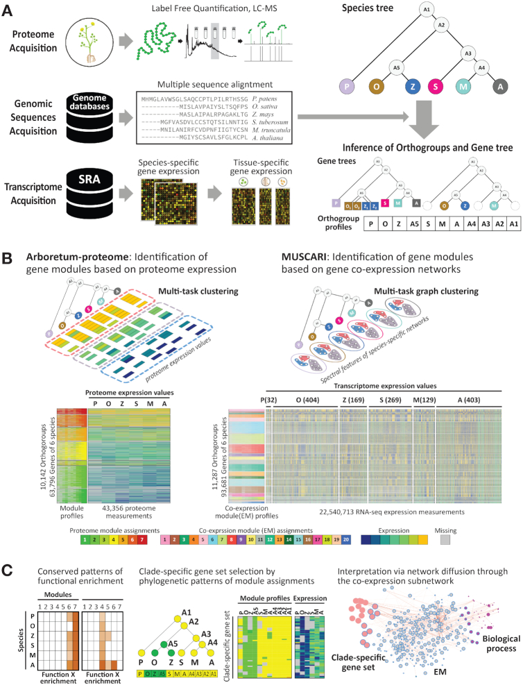
Overall approach of comparative analysis. The overall framework of our comparative analysis has three parts: data acquisition, inference of modules and interpretation of modules and gene sets. (A) Input data for the comparative approach includes quantitative proteome measurements for each the six plant species (P. patens, O. sativa, Z. mays, S. tuberosum, M. truncatula, A. thaliana), RNA-seq expression compendium for each species obtained from SRA using Curse/Prose suite, and species phylogenetic tree and genome sequences used for learning gene trees using OrthoFinder. (B) Module identification. Module identification was based on two multi-task clustering algorithms, Arboretum-proteome and Muscari. Arboretum-proteome infers gene modules from proteome data (left). Muscari infers gene co-expression modules mRNA levels (right). Both algorithms use measured data at each species node and phylogenetic relationships while inferring these modules. The heat maps under each algorithm cartoon show the module identification result: module ID profiles are the inferred module assignments (designated as various colors) and the corresponding measured values reordered by each module. The numbers in parenthesis on top of the Muscari output show the number of RNA-seq samples used in Muscari module identification. (C) Analysis and interpretation entails testing modules for enrichment of curated gene sets, identification of gene sets with interesting patterns of conservation and divergence and further annotating them based on enrichment and network diffusion proximity to curated gene sets. Abbr. for species. P: P. patens, O: O. sativa, Z: Z. mays, S: S. tuberosum, M: M. truncatula, A: A. thaliana).
To allow comparison of functional genomic profiles such as proteomic levels across multiple species, we applied two multi-task clustering algorithms. The first algorithm, Arboretum-proteome, is based on Arboretum to infer the modules of the extant species and their ancestral nodes on the phylogenetic tree based on a small number of measurements from multiple species. The resulting module assignment inferred by Arboretum-proteome enables us to trace the evolutionary trajectories of changes in expression level of genes and define clade-specific gene sets exhibiting different patterns of phylogenetic conservation. The second algorithm, Muscari, enables comparison of RNA-seq co-expression modules across species, which are then used to interpret the conservation and divergence relationships at the protein levels. Both algorithms also used input gene trees which explicitly model gene duplication and losses, a major mechanism of evolutionary divergence (43–47). For input data of Muscari, we collected RNA-seq data for the six species from Sequence Read Archive (SRA) (26) to create a species-specific gene expression compendium by using the Curse and Prose suite (27). Finally, to interpret the modules and gene sets, we tested them for enrichment of known and curated gene sets and co-expression modules identified Muscari. We applied our approach to the proteomic dataset collected in this study to examine the patterns of conservation and divergence of protein levels globally at the level of both gene modules and gene sets, and assessed how these are related to species-specific traits.
Proteome levels diverge with phylogenetic distance
Studies in yeast (1) and mammalian (7) phylogenies have shown that genome-wide mRNA profiles diverge phylogenetically, that is, species that are close on the phylogeny have more similar expression profiles than species that are further apart. To assess this property in our proteomic dataset, we correlated the similarity in protein levels between pairs of species to their phylogenetic distance (Figure 2). Phylogenetic distance was estimated by constructing a phylogenetic tree from protein sequences with branch lengths estimated using PAML (34). The similarity in protein levels for a pair of species was measured using the Pearson's correlation of their respective protein levels of orthologous proteins (Materials and Methods). We compared the correlation and phylogenetic distance with Pearson's correlation (PCC), slope as well as the r2, and found that there is a negative correlation between phylogenetic distance and similarity in protein expression (PCC = −0.73, Figure 2A, B), which suggests that two species which are close to each other on the phylogeny have similar expression patterns of proteins.
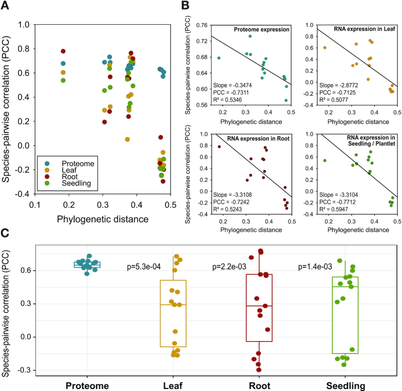
Relating phylogenetic distance to global proteomic and mRNA similarity across species. (A) Scatter plot comparing phylogenetic distance (x-axis) to correlation value (PCC, y-axis) of proteome (blue) or tissue-specific transcriptome expression values (red, green, yellow) for the six species. (B) Scatter plots from the proteome or individual transcriptomes. The linear regression line fit to the scatter is shown. Slope, Pearson's correlation coefficient (PCC) and regression r2 values describing the linear relationship between phylogenetic distance and similarity in proteome (or transcriptome) levels are displayed on the bottom left of each plot. (C) Box plot showing the distribution of correlation values computed for each pair of species using the proteome or transcriptome measurements (dots). t-Test P-value comparing the proteome-based correlation distribution to each of the three transcriptome-based correlation distributions are shown next to the boxplot for each tissue transcriptome.
Next, we corroborated this trend with publicly available transcriptomic measurements in all six species (Figure 2A, B). We used the expression compendium collected for the inference of co-expression modules with Muscari. We selected tissue-specific gene expression profiles from the whole compendium of each species based on their metadata annotation in SRA (Supplementary Table S3, Materials and Methods) and calculated the similarity in gene expression levels for a pair of species by using Pearson's correlation in the same way as protein expression. In particular, we used the same number of orthogroups used for the protein level correlations. We observed a similar anti-correlation from the tissue-specific expressions of leaf, root, and seedling, ranging from PCC = −0.71 to −0.77 (Figure 2B) as well as in other tissues which were available in subsets of our six species (Supplementary Figure S4A), which suggests that two species that are closer to each other in phylogenetic distance have more similar levels of expression. Furthermore, we confirmed this correlation was not an artifact of the number of genes by considering different subsets of genes (Supplementary Figure S4B) and the number of mRNA samples available for a tissue in a species (Supplementary Figure S13). Across species, moss had lowest correlations, which could be due to imperfect matching of moss tissues with the other species.
Overall, both protein and tissue-specific gene expression exhibited a negative correlation, which is consistent with previous studies of expression divergence in mammals (7) and smaller scale studies in plants (13). Although both transcriptome and proteome of two species exhibited an anticorrelation with phylogenetic distance, the pairwise similarities of the proteome were generally higher than those of the transcriptome (Figure 2C). This is also apparent in the lower slope of proteomic divergence versus phylogenetic distance compared to transcriptome divergence versus phylogenetic distance, which suggests that the mRNA levels are less constrained compared to protein levels. This observation is consistent with a previous study comparing mRNA and protein levels in three primate species and found significant changes at the mRNA level without any corresponding changes at the protein level, suggesting that protein levels are under greater evolutionary constraint (12,48). While the proteome-wide analysis of correlations provides a coarse picture of the evolutionary trends, it does not inform us about specific gene modules or pathways that may evolve under different evolutionary pressures. Therefore, we developed and applied a gene module and pathway-based approach that we describe next.
Inference of proteome modules across the plant phylogeny using Arboretum-proteome
To gain insight into the specific processes and pathways that are conserved and diverged in these species at the protein level, we developed Arboretum-proteome to infer groups of proteins with similar protein levels across the six plant species (Figure 3). Arboretum-proteome is a modified version of the Arboretum (23) algorithm, which was initially developed to identify gene co-expression modules at extant and ancestral species using a multi-task Gaussian mixture model while handling complex gene orthologies due to gene duplication and losses (Materials and Methods). Arboretum-proteome learns 1D Gaussian distributions for each group of proteins and assigns the most plausible module membership to all possible ancestral nodes of each gene tree. Arboretum-proteome's multi-task learning framework automatically provides matching between the modules across species. That is module in one species corresponds to module in another species. This matching enables us to easily compare modules across species, which would otherwise require a post hoc matching step.
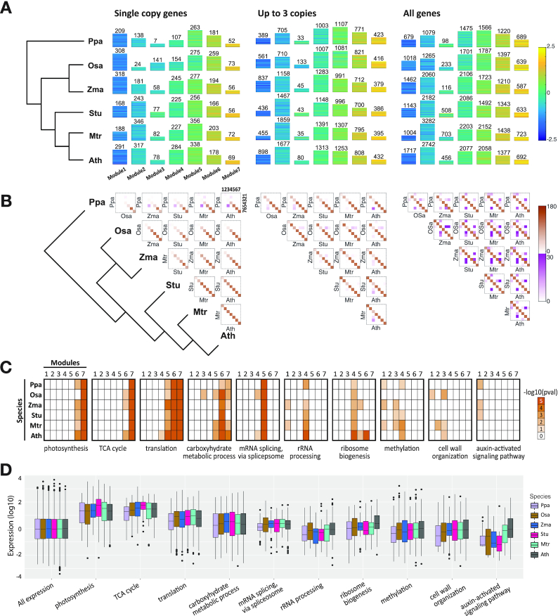
Arboretum analysis of the proteome levels. (A) Gene modules identified from Arboretum-Proteome using three different sets of gene families, which differ based on the gene duplication level: Single copy, Up to three copies and all genes. For each gene family set, seven modules were identified, depicted as yellow-blue heat maps, blue representing low levels while yellow representing high levels. The height of the heatmap corresponds to the number of genes in the module. (B) Plots of orthologous relationship between the seven identified gene modules for each species pair (squares). Diagonal entries correspond to the conservation of matched gene modules between two species, that is they have the same ID, whereas off-diagonal entries assess overlap between modules of different IDs. The intensity of each cell is proportional to the −log(P-value) of overlap. Two colors are used for the heat map because the range of off-diagonal elements is substantially lower than the values for the diagonal elements. (C) Conservation patterns of enriched functional annotations obtained from Gene Ontology (GO). Each heat map shows the enrichment of all seven modules across all species for a particular process, e.g. Photosynthesis, cell wall organization etc. In each subplot, rows correspond to six plant species and columns to module IDs. Different color intensity is proportional to the extent of enrichment. (D) Box plot of the distribution of actual measured proteome values for genes that are annotated with terms mentioned in (C).
We applied Arboretum-proteome to three sets of orthogroups from three different levels of duplication: (i) orthogroups that had no duplication events (4,557 orthogroups, 17,091 genes), (ii) orthogroups with at most three copies of genes (11,587 orthogroups, 66,887 genes) and (iii) all orthogroups with at least two species (15,401 orthogroups, 146,021 genes), and identified seven modules (Methods). We denoted ‘Module 1’ as the module that had the lowest protein levels and ‘Module 7’ as the module that had the highest protein levels (Figure 3A). Despite the considerable phylogenetic distance between the species, we recovered conserved patterns among species and each pattern exhibited roughly the same number of genes. We assessed the extent to which pairs of proteins in a module are co-expressed at the mRNA level and find that protein pairs in most modules are significantly co-expressed compared to background gene pairs (KS test P-value < 0.05), with the exception of the lowly expressed modules from moss and Arabidopsis (Supplementary Figure S14, Materials and Methods).
We next compared the extent to which genes within modules were conserved across species by computing significance of overlap across all pairs of modules from two species (Figure 3B). Matched modules show significant overlap in general (diagonal elements of the heat map), suggesting that proteins with the same expression level tend to be conserved across species. However, the extent of conservation and divergence depends upon the module's protein level: modules with higher expression were more conserved than modules with lower expression. We also observed several significant off-diagonal entries (off-diagonal elements). Such entries represent orthologous genes that have diverged in their protein levels. The extent of divergence between modules increases with phylogenetic distance, with P. patens exhibiting the fewest number of conserved modules, and the eudicots (M. truncatula, A. thaliana, S. tuberosum) showing the most significant conservation among themselves. Module divergence is most consistent with the phylogeny for the single copy gene set. In particular, when considering the ‘single copy’ gene set, only moss exhibited divergence in Modules 5 and 2 compared to other species. The number of substantial off-diagonal entries increases with the extent of duplicated gene groups, although still maintaining an orthologous core, suggesting that duplicated genes contribute to the divergence of gene modules.
To identify the biological processes associated with each module, we tested the modules of all six species for enrichment of species-specific Gene Ontology Biological Process (GO-BP) terms (36) (Figure 3C, D) and KEGG pathways (42) (Supplementary Figure S15). We found that each module had a considerable number of significant associations with specific GO processes and several of these terms are conserved across all six species. In particular, the highly expressed gene modules (modules 6 and 7) are associated with generic biological processes (Figure 3C) such as photosynthesis, TCA cycle (module 7), translation (modules 6, 7). The association of these processes with the highly expressed modules is conserved across the phylogeny, which is also consistent with our observation that modules that are highly expressed are most conserved. Modules with intermediate levels of expression (modules 4 and 5) also exhibit conserved enrichment, albeit to a lesser extent. For example, module 5 is enriched for ‘mRNA splicing, via spliceosome’ which is conserved across all species, while module 4 is enriched for ribosome-related processes. In contrast to the high and medium expressed modules, modules associated with low expression (modules 1, 2 and 3) exhibit the least level of conservation pattern and are associated with post translational modification processes such as ‘methylation’, signaling pathways (‘auxin-activated signaling pathway’) and several minor metabolic and catabolic processes (‘lipid catabolic process’ and ‘cell wall organization’). This analysis suggests that core processes such as photosynthesis are conserved and highly expressed in all the species compared, while regulatory processes (post-translational modifications and signaling pathway) are more diverged. We confirmed this observation by examining the distribution of measured protein levels for each of the selected terms in all the species (Figure 3D). The protein levels of genes annotated with photosynthesis and TCA cycle are significantly higher than the levels of proteins annotated with posttranslational modification processes. We observed a similar trend with KEGG pathways (Supplementary Figure S15), several of which agreed with the GO processes.
Taken together, our results suggest that the modules of highly-expressed proteins are conserved in gene content and enriched for generic metabolic processes likely important for all plants (e.g. photosynthesis), whereas less-expressed modules are more divergent and enriched for processes such as post-translational modification and signalling that could regulate the proteome level in a species, tissue and condition-specific manner.
Clade-specific gene set identification based on divergent patterns of profiles
Our analysis so far examined the conservation patterns of entire modules of genes. To gain insight into genes that exhibit specific phylogenetic patterns of divergence (e.g. upregulated in one clade but not in the other), we next identified clade-specific gene sets, defined as genes that change their modules or are lost or gained across the phylogeny in a clade (e.g. monocots versus eudicots) or species-specific manner. That is, such genes could be either those that have orthologs in a different species but have diverged at the protein level (indicated by switches in module assignment), or genes that have been lost. To identify such genes and groups of genes, we generated the profile of module assignments along the phylogeny for each gene (six extant and five ancestral points, Figure 1A) and analyzed these profiles using two strategies: rule-based approach and de novo clustering.
Our rule-based approach used filtering rules to check if there were genes assigned to highly induced or repressed modules in specific clades (Materials and Methods). We identified 23 gene sets that exhibit clade-specific high or low expression in different clades (Supplementary Table S5). Our de novo clustering approach applied hierarchical clustering on the module profiles to detect gene sets that have similar patterns in a more unbiased manner (Materials and Methods). Our analysis identified 286 gene sets spanning 6,979 of the total 15,401 orthogroups including 42,026 genes across all six species (Supplementary Table S5). These gene sets exhibited three types of patterns: (i) complete conservation in a module assignment across all species, (ii) loss in some species but conserved in others, (iii) changes in module assignments or loss. Of these (ii) and (iii) represent clade-specific gene sets that have either a gene loss or change in module assignment. The majority of the gene sets exhibited the type (ii) pattern of loss in some species but conserved module assignment, or small changes in module assignments, indicating divergence between modules with adjacent levels of protein expression.
To assess the quality of these gene sets we carried out several large-scale analyses. We first tested the 309 gene sets comprising the 23 rule-based and 286 de novo sets for support of co-expression (Supplementary Figure S16). In other words, we asked if pairs of genes in a clade-specific gene set were significantly co-expressed at the mRNA level, considering mRNA measurements across all species, compared to background gene pairs (see Materials and Methods). Of the 23 clade-specific gene sets, 11 were significantly co-expressed (KS test P value < 0.05), while of the 286 de novo sets, 101 were significantly co-expressed. Next, we tested each gene set for enrichment of GO processes by first projecting them into species-specific gene sets and tested the significance of overlap of the gene set with annotated genes of a GO process. In each species, a substantial number of gene sets were enriched for a GO process (Supplementary Table S5). Between 7–14 gene sets per species were enriched for different biological processes (FDR<0.05) resulting in a total of 17 gene sets enriched in any species (Figure 4A). Of the 286 gene sets, between 38–83 gene sets are significantly enriched in different biological processes, with P. patens exhibiting smallest number of gene sets enriched, which is expected as it had the greatest extent of losses (Figure 4A). To investigate the large-scale patterns in the enriched processes of the clade-specific gene sets, we applied Non-negative Matrix Factorization (NMF)-based bi-clustering to group both gene sets and the associated process terms into 10 groups and characterized the process group by highest scoring term for the cluster (Figure 5 and Supplementary Table S5). The process groups capture different classes, including cell wall biogenesis, metabolism, transport, signaling, photosynthesis and oxidation reduction (Figure 5). Interestingly the gene sets within a group associated with a specific group of processes had different patterns of proteome conservation, e.g. gene set 1013, 1056, 990, in group 5, suggesting the gene sets capture more fine-grained structure of a GO process. The GO analysis provides support for our results but also suggests that different parts of the process of interest might experience different evolutionary forces.
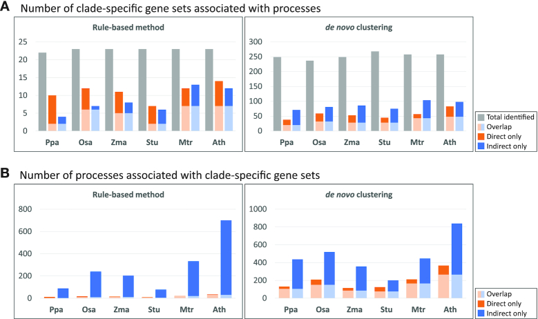
Association of clade-specific gene sets with GO processes. (A) Number of clade-specific gene sets from the rule-based approach and de novo clustering that are associated with GO processes based on ‘direct’ enrichment (FDR, P<0.05, orange bar) or ‘indirect’ association based on network diffusion-based connectivity (Mann–Whitney Wilcoxon test, P < 0.05, FDR < 0.1, blue bar). The light blue and light orange parts of the bar indicate gene sets with both direct and indirect enrichment. Total number of gene sets identified from each species is depicted as grey bars. (B) Number of GO processes enriched in clade-specific gene sets from the rule-based approach and de novo clustering based on direct (orange bar) or indirect method (blue bar). Light blue and orange bars indicate processes identified by both approaches of term association.
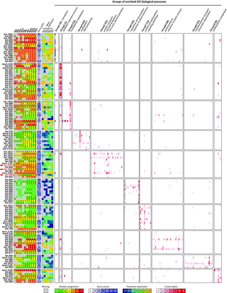
Non-negative matrix factorization (NMF) analysis of enrichment patterns of clade-specific gene sets. The enrichment of 125 clade-specific gene sets (17 rule-based, 108 de novo, rows) for 186 GO processes (columns) was designated as a matrix where each entry is the number of species that showed enrichment in a process. The matrix was clustered into 10 groups by NMF and re-arranged based on the cluster assignments. For each gene set, the proteome module ID profiles (first set of columns), the number of genes (second column) and the mean proteome expression values across genes (third set) is shown. For each of the 10 groups of GO processes, the number of processes (in parenthesis) and the representative GO process term is shown. Intensity of red is proportional to the number of species with the enrichment. The specific gene sets that are mentioned in the main text are indicated with red arrows and red font. Abbr. for species.Ppa: P. patens, Osa: O. sativa, Zma: Z. mays, Stu: S. tuberosum, Mtr: M. truncatula, Ath: A. thaliana, Anc1–5: ancestral points)
Taken together, our de novo and rule-based methods of identifying clade-specific gene sets were able to predict meaningful gene sets that are indicative of the evolutionary dynamics of gene groups, are supported by co-expression at the mRNA level and enriched in different biologically processes that are helpful to study species and clade-specific adaptations.
Integrating mRNA co-expression modules across the phylogeny to interpret clade-specific gene sets
While the interpretation of clade-specific gene sets based on significant overlap of curated gene sets such as gene ontology was useful, we were able to interpret only a small fraction of our de novo gene sets (Figure 4A). This is because many of our genes are poorly annotated. This is limiting because we had several clade-specific gene sets with interesting patterns of module divergence or loss, but we could not associate a possible biological pathway to them. To expand the scope of our clade-specific gene sets to more molecular pathways and processes, we turned to publicly available gene expression compendia of these species. Gene expression modules defined by co-expression signatures of genes across different spatial and temporal conditions are often associated with specific molecular processes and pathways and therefore offer a robust basis to interpret gene sets identified using complementary experimental techniques. Hence, we defined expression modules to enable the interpretation of more of our clade-specific gene sets. We included all available spatiotemporal expression data but excluded data from mutant, knock out and transgenic lines. As a result, we were able to construct a compendium consisting of at least 32 experiments (P. patens) up to 404 experiments (O. sativa), which cover more than 99% of the genes in all six species’ proteome. We used the expression data of each species to construct species-specific genome-wide co-expression networks (Materials and Methods).
To define expression modules jointly across the six species, we developed a multi-task graph-clustering algorithm, Muscari (MUlti-task Spectral Clustering AlgoRIthm, Methods). The input to Muscari are weighted graphs, e.g. co-expression networks, one for each leaf node and phylogenetic relationships (species and gene trees). Muscari uses both the phylogenetic relationship between species and the co-expression networks to define co-expression modules across species. This strategy allows us to identify matched modules across species and has a significant benefit over independent clustering of co-expression networks, which would require post-processing to carry out additional comparative analysis (49). Using Muscari on the transcriptome compendia, we learned k = 20 Expression Modules (EMs) consisting of at least 49 genes (P. patens ‘EM19’) and up to 3,725 genes (M. truncatula ‘EM6’, Supplementary Table S6). All 20 modules were enriched for diverse biological processes that included generic (e.g., DNA repair in EM17, response to stress in EM2, translation and ribosome biogenesis in EM3), as well as plant-specific terms (Supplementary Table S6) that were conserved across the entire phylogeny (e.g. photosynthesis in EM1, chloroplast organization in EM5) or exhibited species-specific divergence (e.g. leaf vascular tissue pattern formation in EM8 in Arabidopsis and Medicago).
Since each EM specifies subnetworks of possible biological contexts determined by the constituent genes, we leveraged the EMs for functional annotation and interpretation of our clade-specific gene sets. Briefly, we hypothesized that if the association between the clade-specific gene set and a biological process is valid, then genes in the clade-specific set should be more strongly connected to the genes in the process of interest than other genes in the network. We first tested each clade-specific gene set for significant overlap with an EM using a hyper-geometric test (FDR < 0.05) and putatively associated all the GO processes enriched in the EM to a clade-specific gene set with which it had significant overlap (Methods). Next, to test the associations of GO processes to clade-specific gene sets, we applied network-based information propagation from a clade-specific gene set to all other genes to assess their global connectivity on a gene network (50). If a clade-specific gene set had significantly higher diffusion scores (higher connectivity) for the genes annotated with a GO process compared to other genes, we considered that as a validated association. Across the species, 4–13 out of 23 rule-based gene sets were enriched in 15 EMs and 71–104 out of 286 de novo gene sets were enriched in 18 EMs (Supplementary Table S7). Based on the network diffusion, we annotated 47–61 additional de novo gene sets and 1–6 rule-based gene sets across species that were associated with 201–839 processes across the six species (Figure 4). Of these processes, between 125 and 574 were specifically based on the network-based diffusion.
We found a substantial increase in the proportion of the de novo gene sets associated with a specific biological process (Figure 4A). This suggests that although the genes in the clade-specific set are not directly annotated with a process, they are strongly connected to the genes annotated with the process. Several of these ‘gene set - GO biological process’ relationships are visually apparent on the co-expression graph (Figure 6, Materials and Methods). For example, the gene set 1013 significantly overlaps EM11 (Figure 6A), which is further enriched for the process ‘maintenance of root meristem identity’. Visualization of these genes on a network shows that genes annotated with ‘maintenance of root meristem identity have higher node values (bigger node sizes, Mann–Whitney Wilcoxon (MWW) test P < 0.05) than genes annotated with ‘seed germination’ (P = 0.979, MWW test), when considering the connectivity to gene set 1013.
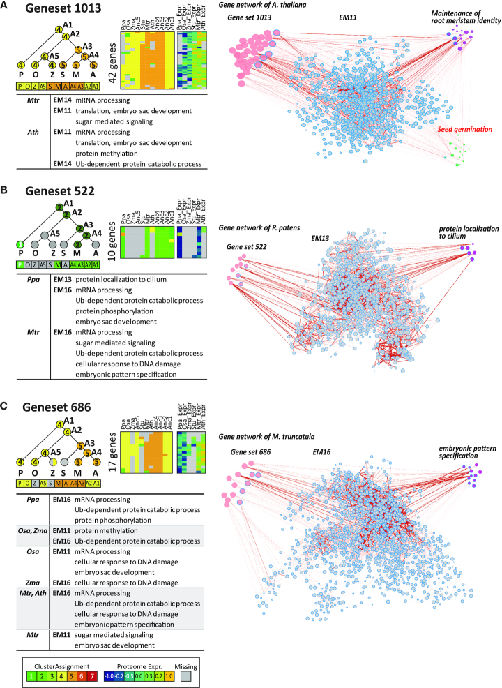
Clade-specific gene sets associated with a GO process based on network diffusion. On the left is the phylogenetic pattern of the gene set, followed by the heatmap showing module assignments and protein levels for the gene set of interest. The right part of each panel shows the co-expression network with nodes proportional to the diffusion score from the input gene set. Each network consists of clade-specific gene set (red nodes), Muscari expression module (EM; blue border outlined nodes), and genes annotated with specific biological processes (purple nodes). Thickness of edges corresponds to the edge-weights of co-expression network. Associated processes are summarized in the table at bottom. (A) Gene set 1013. Note that genes annotated with an unrelated term (‘seed germination’ in red font) shows smaller node size (green nodes) and weaker edge weights. (B) Gene set 522, (C) Gene set 686.
Several clade-specific gene sets exhibiting induction or depletion of protein levels in specific clades were associated with biological processes likely important for that species or clade based on their association with EMs (Figure 6, Supplementary Figure S17). For example, the gene set 522 was upregulated in P. patens compared to the other species (Figure 6B) and was enriched for expression module EM13 of P. patens, and predicted to have a role in ‘protein localization to cilium of motile sperm’ (P < 0.05, MWW test), which is likely a P. patens specific function. We found several additional gene sets that were induced in P. patens (gene sets 670 and 975, Supplementary Figure S17B), that are likely associated biosynthesis of secondary metabolites such as vitamin B6 (EM4 of P. patens, gene set 670) and protein modification such as protein phosphorylation (EM16 of P. patens, gene set 975) based on their association with different EM modules. Several gene sets specifically induced in eudicots did not have a direct GO enrichment, but are associated with different GO processes based on their connectivity to an EM module. For example, gene set 686 significantly overlaps EM16 (Figure 6C), which contains genes associated with ‘embryonic pattern specification’ explicitly in M. truncatula and A. thaliana, which suggests these genes could be involved in species-specific embryonic development.
The network diffusion step greatly expanded the number of GO processes associated with the clade-specific gene set enabling us to associate our clade-specific gene sets to hundreds of GO process (Figure 4B). To identify the large-scale patterns of these GO enrichments, we applied the same matrix factorization-based bi-clustering approach (Figure 5) to obtain groups of GO terms and gene sets (Supplementary Figure S11). There was a clear grouping of gene sets by terms, but each set of terms was more diverse than the directly enriched GO processes. Nevertheless, annotating each term group based on the most high-scoring term identified a variety of processes including post-translational modifications, chromatin remodeling, photosynthesis, secondary metabolite processes and cell cycle related processes. Taken together, by using the co-expression network and network diffusion we were able to expand the interpretation of our clade-specific gene sets to additional biological processes that could be impacted by evolutionary changes at the protein expression level.
Clade-specific gene sets link rhizobia-legume symbiosis to autophagy-related processes
Our rationale for identifying clade-specific gene sets was that they can be used to identify genes that are associated with species-specific traits. As a case study, we considered the rhizobium-legume symbiosis (nodulation) pathway, as our species panel includes a species that can form this symbiotic relationship (M. truncatula) with rhizobia as well as species that do not. We first examined four curated gene sets: (i) genes known to be involved in root nodulation and symbiosis (nodulation1), (ii) genes involved in root nodulation and nitrogen fixation (nodulation2), (iii) genes involved in mycorrhizal associations that often share common mechanisms with nodulation (mycorrhizal_assoc) and (iv) genes frequently lost in non-mycorrhizal lineages (lost_in_non-mycor), likely playing a role in mycorrhizal associations and possibly, by extension, in some aspects of the rhizobium-legume symbiosis (51) (Supplementary Table S8). We first traced their module assignments and found that they are not localized to a specific module (Figure 7A). As expected, species such as P. patens and A. thaliana, which are known to lack the ability to form symbiotic relationships exhibited a large amount of loss for these gene sets. Interestingly, if an ortholog for M. truncatula was present, in the majority of the cases its module assignment was preserved. This pattern is generally true for genes analyzed in our study, where we see that if a protein is measured in a species, the protein module assignment is usually the same. There are a few notable exceptions that are associated with monocot/eudicot divergence, as well as P. patens-specific behavior.
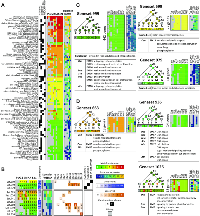
Analysis of nodulation related genes and processes. (A) Genes known to be associated with nodulation in M. truncatula based on four different sources. Rows are Medicago genes. First set of white-black columns depict binary membership of genes in four curated gene sets: nodulation1, nodulation2, mycorrhizal_assoc, lost_in_non-mycorrhizal species. Second set of columns show the inferred module assignment at the extant and ancestral points. The third set of columns show the proteome levels of the genes. (B) Clade-specific gene sets defined from de novo clustering which are related to nodulation either by direct overlap with curated gene sets or based on their overlap with Muscari expression modules (EMs) enriched for nodulation related processes. The first group of columns shows the proteome module assignment profile. Species abbreviations: P: P. patens, O: O. sativa, Z: Z. mays, S: S. tuberosum, M: M. truncatula, A: A. thaliana. The second column shows the gene count in each gene set. The third set of columns show the mean proteome expression values across genes in the gene set. The remaining groups of columns show the EMs or nodulation gene set with significant overlap. (C, D) Examples of gene sets that are directly enriched (C), or indirectly associated based on significant network diffusion scores (D). Each panel shows the phylogenetic pattern of the gene set, the module assignments (6 colors), the protein levels and GO processes associated with gene set based on network diffusion (Figure 6A). For (C), the curated nodulation gene set enriched in the clade-specific set is listed.
Next, we investigated our clade-specific gene sets for their relationship to these nodulation-related gene sets by testing them for overlap of either (a) the nodulation gene sets or (b) an EM enriched for these nodulation gene sets or nodulation related GO process (Figure 7B). Three of our clade-specific gene sets (gene sets 599, 979 and 999, Figure 7C) are enriched for the curated gene sets, namely, gene set 599 is enriched for the genes frequently lost in non-mycorrhizal species (lost_in_non-mycor), and gene set 999 is enriched for the nodulation2 set. These gene sets include the original genes annotated with these processes but also contain additional genes with similar phylogenetic trends. Integrating the expression modules further helps to interpret these gene sets (Figure 7B, top). For example, both gene set 599 and 999 exhibit association with the GO process ‘autophagy’ via EM13 of O. sativa. Autophagy likely plays an important role in controlling the colonization of nodule cells by functional bacteroids as autophagosomes were observed in the nodule cells of dnf1 mutants (52). The role of autophagy-related proteins in the establishment of symbiotic relationships has been also observed in Phaseolus vulgaris (53), which showed that down-regulation of an autophagy-related kinase significantly inhibited the ability of P. vulgaris to form root nodules. Moreover, gene set 599 which was enriched for the lost_in_nonmycor gene set (51,54) is also enriched for ‘cellular response to nitrogen starvation’ (P = 8.1e–8) via O. sativa EM13 (Figure 7C). Nutrient limitation is a key environmental signal that controls the establishment and the maintenance of the mycorrhizal associations (55).
To find additional genes and pathways associated with nodulation, we examined the M. truncatula EMs enriched for these curated gene sets and nodulation related GO processes, such as ‘nodulation’ and ‘response to bacterium’. We found several M. truncatula EM modules enriched for these processes (nodulation: EM19, response to bacterium: EM7) and curated gene sets (nodulation1: EM13, nodulation2: EM19, lost in non-mycorrhizal species: EM17 and EM19). We next obtained clade-specific gene sets enriched in these EM modules and identified eight additional gene sets (Figure 7B, bottom). Genes in these sets are always present in M. truncatula and have a tendency of low protein expression state except gene set 663. Among these, gene set 936 (Figure 7D) was particularly interesting because it was enriched in EM17, which was further enriched in ‘sugar mediated signalling pathway’. A recent study in soybean suggests that sugar mediated signalling can act as a regulator in nodulation (56,57). Another gene set 1026, which has induced protein expression in M. truncatula and Z. mays, significantly overlapped EM7 of O. sativa, Z. mays and M. truncatula, which are all mycorrhizal species. EM7 is enriched for processes such as ‘cell surface receptor signalling pathway’, ‘signal transduction by protein phosphorylation’ and ‘response to ethylene’ in these species, which suggests that gene set 1026 is likely related to the molecular signal transduction of nodulation. Finally, gene set 663 is also interesting as it is upregulated in M. truncatula, Z. mays and O. sativa and lost or downregulated in P. patens and A. thaliana respectively. It is enriched in EM13, which as discussed above is associated with autophagy.
Taken together, our integrated pipeline of identifying clade-specific gene sets and interpreting them based on enrichment in curated gene sets and EMs enabled us to identify meaningful relationships between different processes and the nodulation phenotype of interest and predicted additional pathways that may be involved in nodulation.
DISCUSSION
Comparative functional genomics offers a powerful lens into the molecular changes associated with diverse species-specific traits and has been used to study transcriptome evolution in different yeast and mammalian species. Recent advances in high-throughput mass spectrometry (MS) are enabling comparative proteomic studies across multiple species (12). However, measuring proteomic profiles in plants remains challenging because of the large number of proteins and high dynamic range. Furthermore, systematic comparison of proteins levels across numerous species and interpretation of patterns of conservation and divergence in the context of specific biological processes is a significant challenge in plant phylogenies, which have substantial duplication events and are not as well annotated as mammalian species.
In this study, we optimized an MS-based assay to measure the proteomes of six plant species and developed a computational pipeline to compare and interpret these proteomic measurements across the species. Global comparison of protein levels suggests that proteome divergence is proportional to phylogenetic distance. Furthermore, the protoeme is more constrained than the transcriptome from different tissues, which is consistent with studies in mammals (7). Our pipeline leverages multi-task clustering algorithms, Arboretum-proteome and Muscari, that jointly examine multiple species-specific datasets while incorporating phylogenetic information to identify groups of conserved proteins and gene subnetworks. Such gene groups can provide insight into specific molecular processes and pathways that can contribute to species-specific traits. Using our integrated approach, we identified several clade-specific gene sets and linked them to different biological processes that exhibit species-specific divergence.
There are relatively few studies that have compared proteomes of species, especially plants. While this work was in review, a study comparing 13 plant species was published (21). The goals of this study and ours was different; this study aimed to identify conserved proteome interaction complexes using a co-elution method to detect complexes, whereas we identified conserved proteome modules with proteins with the same level of expression. We correlated the co-expression levels of proteins in the three species present in both studies and found a good correlation of 0.52–0.59. We also compared the orthology relationships between the two studies and found a high overlap (Jaccard index of 60%, Materials and Methods). Overall, despite different technologies and processing pipelines, the two datasets are comparable.
Our analysis showed that highly expressed proteins are more conserved than proteins expressed at lower levels. Highly expressed proteins are associated with ubiquitously important processes such as photosynthesis, whereas gene modules that have low protein expression level tend to be enriched for regulatory processes (e.g. post-translational modification). This observation is consistent with core metabolic processes being universally conserved while regulatory processes being involved in driving species-specific behavior. Our observation of divergence in regulatory processes are supported by several existing studies which have focused either on individual cells for yeast (58) comparing the proteome and transcriptome of a single yeast strain, or compared the transcriptome across multiple species (59). One caveat in the analysis is that lowly expressed proteins are also hard to measure and poorly annotated in the genome. That is, they could be present but are not detectable by current experimental assays, which in turn can influence our annotation assembly. Hence, for lowly expressed proteins, it might be difficult to discern whether the divergence is due to loss or due to the change in protein levels between species. In our current study, we address this issue by examining the patterns of conservation against permuted gene sets (Supplementary Figure S18) and requiring multiple species (e.g. a group in a clade) to exhibit a particular change or loss of gene. By requiring multiple species to vote on a specific pattern of expression in a clade, we are less susceptible to spurious losses or module changes. As more species can be added to these datasets, a more complete and accurate study of loss and divergence can be performed.
A significant challenge in the analysis of high-throughput data, especially in understudied organisms, is the validation and interpretation of the results. In our setting, we identified several clade-specific gene sets that exhibited a phylogenetically interesting pattern of protein level change or loss. Using standard gene ontology and KEGG pathway annotation we were able to interpret only some of these gene sets, but the vast majority were not directly associated with a particular process. To address the challenge of interpreting these gene sets, we used large-scale expression compendia to derive expression modules and co-expression networks. Our rationale was that if our groups of clade-specific genes are valid, they should have support at the co-expression level. Using Muscari, a multi-task graph clustering approach, we defined co-expression-based gene modules, which had significant overlap with several of our gene sets. Furthermore, these co-expressed genes were enriched in additional processes that allowed us to predict potential process associations for our clade-specific gene sets. This approach provides a general strategy to examine other processes and phenotypes of interest within an evolutionary framework.
Our comparative integrative framework is related to several existing approaches in the field, although they are not directly applicable because of the complex orthologies in our dataset. One approach, MINT (60) aims to define common signatures across different datasets measuring the same genes. Such datasets are gene expression datasets and MINT proposes a partial least square regression approach to project the datasets into a shared space while also determining the key variables that drive the differences between the datasets. In our approaches, Arboretum-Proteome and Muscari, we too have multiple datasets that we jointly analyze to define key signatures of conservation and divergence. However, our datasets are more complicated because of the lack of the one-to-one mapping of genes across species. Another approach by Bodien et al. (61), aims to incorporate longitudinal relationships between microbiome and other omic data. The longitudinal aspect is related to how we model tree relationships between different datasets, while the integration of multi-omic measurements with different sample size distribution is related to the integration of transcriptomic co-expression networks with Arboretum modules. However, the Bodien et al.’s integrative approach is more suitable when the number of measurements in each time point is sufficiently high and there is good correspondence between the samples being measured. Our set up is more challenging as we have only one measurement per species at the protein level and the expression data are publicly available datasets collected from independent studies. Furthermore, as in MINT, one-to-one correspondence is expected between time points. Extensions based on these approaches are promising directions of future work for multi-species multi-omic datasets.
The goal of comparative studies is to understand how changes at the molecular level are associated with changes at the phenotype. Our multi-species proteome dataset is a rich resource that can be used to study processes and pathways driving phenotypic divergence. We used rhizobia-legume symbiosis as a case study to demonstrate the utility of our approach and this dataset. Interestingly, we found that in non-nodulating species, these genes are likely involved in stress response or autophagy-related processes.
Our work can be extended in many ways. The current proteome dataset was using whole plant extracts, and this provided limited insight into tissue-specific patterns of conservation and divergence. New tissue-specific datasets across multiple plant species examined using an approach such as ours could significantly improve our understanding of evolutionary processes driving tissue-specific behavior. Furthermore, measurements of transcriptomes and proteomes from matched tissues across species and integrative analysis of these multi-omic datasets across species would not need the manual matching of tissues across plants as we did in our study and provide novel insight into the tissue-specific evolutionary patterns of the transcriptome and proteome. Hence another direction is to collect matched proteomic and transcriptomic datasets and analyze them using an extended version of our comparative framework that can handle multi-omic datasets. Methodologically, we have considered a spectral clustering approach to jointly define co-expression modules. Graph clustering of the co-expression networks could be considered as a network embedding problem (62), that transforms the input network into a lower dimensional dataset such that the data points are close with respect to an input distance. Another direction of work would be define a joint embedding framework to account for the multi-species nature of our datasets that could handle complex orthology relationships.
In summary, we have created a novel multi-species proteomic dataset spanning a large phylogenetic distance and a suite of computational tools to analyze and interpret this dataset. Our framework can be readily applied to more massive compendia of measurements as they become available and can be useful to link changes at individual proteins and groups of proteins to downstream phenotypes.
DATA AVAILABILITY
The full list of results including identified modules, gene sets, enrichment results, and input data of the analysis including processed proteome, transcriptome and co-expression network data that support the findings of this study are freely available in Mendeley Data at http://dx.doi.org/10.17632/bwzdv623xn. The code and scripts of multi-task clustering algorithms for this study are available via the GitHub repository: Arboretum-proteome (https://github.com/Roy-lab/Arboretum2.0/tree/Arboretum-proteome), Muscari (https://github.com/Roy-lab/Muscari). The scripts of rule-based approach and de novo clustering for defining clade-specific gene sets are openly available via GitHub repository (https://github.com/Roy-lab/clade-specific_gene_sets). The mass spectrometry proteomics data have been deposited to the ProteomeXchange Consortium via the PRIDE partner repository with the dataset identifier PXD013606.
SUPPLEMENTARY DATA
Supplementary Data are available at NAR Online.
FUNDING
National Science Foundation [1546742 to M.S., J.M.A., J.C., S.R.]; National Science Foundation [DBI-1350677 to S.R.]; James McDonnell Foundation [3194-133-349500-4-AAB5159 to S.R.]; Agency for Innovation by Science and Technology (IWT) in Flanders (to D.V.); Basic Science Research Program through the National Research Foundation of Korea (NRF) funded by the Ministry of Education [2019R1A6A3A12033291 to J.S.]. Funding for open access charge: National Science Foundation and James McDonnell foundation.
Conflict of interest statement. None declared.
REFERENCES
1.
2.
3.
4.
5.
6.
7.
8.
9.
10.
11.
12.
13.
14.
15.
16.
17.
18.
19.
20.
21.
22.
23.
24.
25.
26.
27.
28.
29.
30.
31.
32.
33.
34.
35.
36.
37.
38.
39.
40.
41.
42.
43.
44.
45.
46.
47.
48.
49.
50.
51.
52.
53.
54.
55.
56.
58.
59.
60.
61.