 Rampant False Detection of Adaptive Phenotypic Optimization by ParTI-Based Pareto Front Inference
Molecular Biology and Evolution


- Altmetric
Organisms face tradeoffs in performing multiple tasks. Identifying the optimal phenotypes maximizing the organismal fitness (or Pareto front) and inferring the relevant tasks allow testing phenotypic adaptations and help delineate evolutionary constraints, tradeoffs, and critical fitness components, so are of broad interest. It has been proposed that Pareto fronts can be identified from high-dimensional phenotypic data, including molecular phenotypes such as gene expression levels, by fitting polytopes (lines, triangles, tetrahedrons, and so on), and a program named ParTI was recently introduced for this purpose. ParTI has identified Pareto fronts and inferred phenotypes best for individual tasks (or archetypes) from numerous data sets such as the beak morphologies of Darwin’s finches and mRNA concentrations in human tumors, implying evolutionary optimizations of the involved traits. Nevertheless, the reliabilities of these findings are unknown. Using real and simulated data that lack evolutionary optimization, we here report extremely high false-positive rates of ParTI. The errors arise from phylogenetic relationships or population structures of the organisms analyzed and the flexibility of data analysis in ParTI that is equivalent to p-hacking. Because these problems are virtually universal, our findings cast doubt on almost all ParTI-based results and suggest that reliably identifying Pareto fronts and archetypes from high-dimensional phenotypic data are currently generally difficult.
Introduction
The fitness of an organism in an environment is a function of its performances of multiple biological tasks. For example, the fitness of a microorganism rises with its abilities to reproduce given the resource and to acquire new resources when the given resource is exhausted, and the relative contributions of the two abilities to fitness are environment-dependent (Yi and Dean 2016). However, no phenotype can be optimal for all tasks. Fish whose eggs are larger lay fewer eggs (Duarte and Alcaraz 1989). The showy peacock tail attracts mates as well as predators (Darwin 1859). A speedy translational elongation ensures efficient protein synthesis but sacrifices the quality of the proteins synthesized (Yang, Chen, et al. 2014). The concepts of Pareto optimality and Pareto front, borrowed from engineering and economics, help analyze such tradeoffs. In a given environment, Pareto optimality refers to the state under which a phenotype cannot be modified so as to improve the performance of any task without worsening the performance of at least one other task, and the Pareto front is the set of Pareto-optimal phenotypes (Shoval et al. 2012) (fig. 1A).

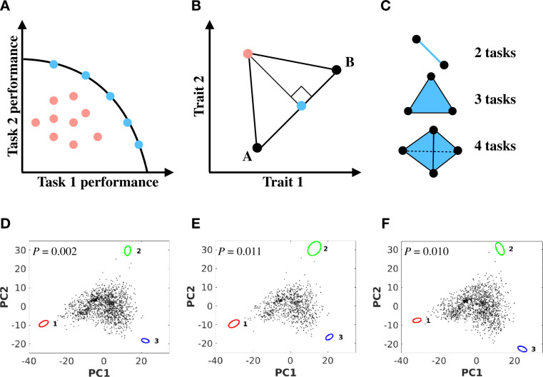
The logic of Pareto front inference and its application to the transcriptomes of yeast gene deletion strains. (A) Natural selection is expected to remove a phenotype (pink) if it is outperformed by another phenotype (blue) at every task. The remaining phenotypes (blue) display tradeoffs in performing the tasks and form the Pareto front. (B) In a phenotypic space, phenotypes A and B are respectively optimal in performing one of the two tasks and are referred to as archetypes. Consider a phenotype x (pink) that is off the line connecting A and B. Its projection on the line, x' (blue), is closer to both A and B than is x so performs better than x in both tasks (see main text). Therefore, any phenotype off the line is outcompeted by its projection on the line. Thus, individuals adapted to their environments will form a line in the phenotypic space. (C) The Pareto front is a line when there are two tasks, a triangle when there are three tasks, and a tetrahedron when there are four tasks. (D) The Pareto front inferred from the transcriptomes of yeast gene deletion strains projected to the first two principal components of the phenotypic space. Each dot represents a transcriptome. The centers of the ovals represent the inferred archetype positions, with the size of the ovals representing the 68% confidence interval of the archetype position obtained by bootstrapping. The P value is the probability that a randomly shuffled data set fits the Pareto front better than the observed data. (E) The Pareto front inferred from the transcriptomes of yeast gene deletions strains less fit than the wild-type. (F) The Pareto front inferred from the transcriptomes of the technical replicates of the yeast wild-type strain.
Identifying the Pareto front and the relevant tasks from a high-dimensional phenotypic data set of a diverse group of organisms is of wide interest to biologists, because it helps verify phenotypic adaptation and offer insights into evolutionary constraints, tradeoffs, key fitness determinants, and the range of natural habitats of the study organisms. It has been proposed that Pareto fronts in a phenotypic space should be polytopes (lines, triangles, tetrahedrons, and so on), and the vertices of these polytopes are archetypes, phenotypes with the best performances of individual tasks (Shoval et al. 2012). This conclusion was drawn on the basis of the following six assumptions: 1) the mapping between a phenotype and the performance of each task is independent of the environment, 2) fitness is an increasing function of the performance of each task, 3) for each task, there is a unique optimal phenotype referred to as the archetype, 4) the performance of a phenotype at a given task worsens as the distance of the phenotype from the archetype of the task increases in the phenotypic space, 5) organisms have evolved to the optimal phenotypes in their respective environments, and 6) the environments of the organisms examined are sufficiently diverse and representative of the organisms’ natural habits.
To see why Pareto fronts are polytopes under the above assumptions, let us consider the case where there are two tasks with the corresponding archetypes of A and B (fig. 1B). For a phenotype x (the pink circle in fig. 1B) that does not lie on the line connecting A and B, we can always find a phenotype x' (the blue circle in fig. 1B) on the above line that is closer than x to both A and B. Based on the above assumptions, x' performs better than x for both tasks, so natural selection will eliminate x. If the organisms examined are from many environments, we expect all observed phenotypes to lie on the line connecting A and B; the exact position of a phenotype depends on the environment where the corresponding organism is sampled because the environment determines the relative importance of the two tasks. This geometric argument can be extended to cases with more than two tasks. The phenotypes should fill a triangle in the case of three tasks and a tetrahedron in the case of four tasks, and so on (fig. 1C). Shoval et al. (2012) used this idea to identify Pareto fronts and associated tasks from various phenotypic data sets, such as the beak morphologies of Darwin’s finches, wing morphologies of bats, and gene expression levels in the bacterium Escherichia coli at different growth stages. The same group subsequently developed a computational method named Pareto-Task Inference (ParTI) for identifying Pareto fronts and archetypes from high-dimensional phenotypic data (Hart et al. 2015). Briefly, ParTI first uses principal component analysis (PCA) to reduce the dimension of a phenotypic data set, where the number of principal components (PCs) considered is arbitrarily chosen by the user. ParTI then applies convex hull fitting algorithms to detect a polytope from the dimension-reduced data; the polytope is regarded as the Pareto front. The Pareto front is considered statistically significant if the dimension-reduced data fit the polytope better than at least 95% of comparable, randomized data. Tasks are then inferred by performing a biological feature enrichment analysis on the vertices of the identified Pareto front.
ParTI is currently the primary computational method for identifying Pareto fronts from biological data and the only method providing a statistical test of Pareto optimality. Numerous Pareto fronts have been reported in the last few years on the basis of ParTI, implying that the relevant traits in various data sets have been evolutionarily optimized. For example, ParTI revealed that animal life-history traits exhibit a triangular Pareto front (Szekely et al. 2015), ammonite shell shapes show a pyramid-like Pareto front (Tendler et al. 2015), the transcriptomes of mouse tissues show a tetrahedron-shaped Pareto front (Hart et al. 2015), the transcriptomes of various cancers have Pareto fronts with three, four, or five archetypes (Hart et al. 2015; Hausser et al. 2019), and single-cell transcriptomes exhibit Pareto fronts with three or four archetypes (Korem et al. 2015; Adler et al. 2019). ParTI and many of the above examples are covered extensively in a new edition of a popular systems biology textbook (Alon 2019), so the concept of Pareto optimality and the method for identifying Pareto fronts will likely become known to more and more researchers interested in phenotypic optimization and adaptation. Because of the increasing availability of high-dimensional data of molecular phenotypes as a result of the rapid advancement of sequencing technologies, ParTI is considered particularly useful in the omics era (Wagner et al. 2016; Hausser and Alon 2020).
Nevertheless, the theoretical prediction that Pareto fronts are polytopes when a set of assumptions are satisfied does not mean that all polytopes are Pareto fronts, because processes other than evolutionary optimization of tradeoffs may also produce polytopes and confound Pareto analysis (Edelaar 2013). These processes must be excluded before Pareto optimality can be established. Unfortunately, despite the popularity of ParTI, factors that potentially confound ParTI have not been systematically studied. In this work, we apply ParTI to real and simulated data of phenotypes that are not optimized, but find that ParTI still detects Pareto fronts and archetypes with a high probability. One source of such false-positive errors is the phylogenetic relationship or population structure among the organisms analyzed, which are unavoidable in many data sets. An even more widespread source of error is the flexibility of ParTI analysis, which forces researchers to make numerous arbitrary decisions in inference. This flexibility makes the ParTI analysis prone to p-hacking, selective reporting of statistically significant results after trying multiple statistical procedures. Our results suggest that Pareto fronts cannot be reliably identified from phenotypic data by fitting polytopes, casting doubt on the validity of ParTI-based Pareto fronts and archetypes so far reported.
Results
ParTI Falsely Detects Pareto Fronts and Associated Tasks from the Transcriptomes of Yeast Gene Deletion Strains
To investigate the performance of ParTI on phenotypic data of organisms that are not adapted to their environments, we analyzed the transcriptomes of 1,484 yeast strains, each with a different nonessential gene deleted (Kemmeren et al. 2014). The gene deletion strains (and their transcriptomes) are apparently suboptimal because they are the products of artificial gene removals from a wild-type strain and would accumulate compensatory beneficial mutations when allowed to evolve in the lab (Szamecz et al. 2014). Furthermore, a number of past ParTI analyses reported Pareto optimality from transcriptomes of bacterial cells at different growth stages as well as transcriptomes of different eukaryotic cells, tissues, and cancers (Hart et al. 2015; Korem et al. 2015; Adler et al. 2019; Hausser et al. 2019). Hence, the transcriptomes of yeast gene deletion strains serve as a suitable negative control for PartTI. We preprocessed the yeast transcriptome data following a recent ParTI study of transcriptomes performed by the authors of ParTI (Adler et al. 2019).
Using ParTI, we found that the transcriptomes of 1,484 yeast gene deletion strains are well described by a triangle (P = 0.002; fig. 1D) with apparently meaningful archetypes (table 1 and supplementary table S1, Supplementary Material online). For example, archetype 1 is best described by mitochondrial functions, archetype 2 is best described by carbohydrate metabolism, and archetype 3 is best described by protein synthesis. We found the ParTI result to remain largely unchanged even after the removal of gene deletion strains that are fitter than the wild-type in the synthetic complete (SC) medium, where the transcriptome data were collected (fig. 1E). Finally, ParTI even identified a significant Pareto front from the 1,484 technical replicate transcriptomes of the same wild-type strain under the SC medium (fig. 1F). The archetypes inferred from the wild-type technical replicates (table 2 and supplementary table S2, Supplementary Material online) are similar to those inferred from the gene deletion strains. Furthermore, the PC coordinates of the wild-type technical replicates are highly correlated with those of the matched gene deletion strains in the microarray experiment (the correlation for PC1 coordinates is 0.96, whereas that for PC2 coordinates is 0.94). Therefore, the false-positive ParTI results found from the gene deletion strains are likely due, at least in part, to spurious signals from the microarray experiment. Clearly, ParTI can falsely detect Pareto fronts from phenotypes that are not Pareto optimal. This alarming finding prompts us to systematically study false-positive errors of ParTI.

| Tasks | Corrected P Values |
|---|---|
| Archetype 1 (mitochondrial function) | |
| Mitochondrial part | |
| Envelope and organelle envelope | |
| Mitochondrial envelope | |
| Establishment of protein localization | |
| Protein transport | |
| Archetype 2 (carbohydrate metabolism) | |
| Gluconeogenesis | |
| Hexose biosynthetic process | |
| Monosaccharide biosynthetic process | |
| Glucose metabolic process | |
| Monosaccharide metabolic process | |
| Archetype 3 (protein synthesis) | |
| Regulation of translational elongation | |
| Regulation of cellular protein metabolic process | |
| Regulation of protein metabolic process | |
| Regulation of translation | |
| Posttranscriptional regulation of gene expression |
Note.—Some P values are identical to each other because of the highly redundant GO annotations of yeast genes. For each archetype, we present five GO categories with the largest median expression differences from the random expectation. The full table is provided in supplementary table S1, Supplementary Material online.
| Tasks | Corrected P Values |
|---|---|
| Archetype 1 (mitochondrial function) | |
| Mitochondrial part | |
| Chromatin organization | |
| Organonitrogen compound biosynthetic process | |
| Envelope and organelle envelope | |
| Mitochondrial envelope | |
| Archetype 2 (carbohydrate metabolism) | |
| Gluconeogenesis | |
| Hexose biosynthetic process | |
| Monosaccharide biosynthetic process | |
| Carbohydrate biosynthetic process | |
| Glucose metabolic process | |
| Archetype 3 (protein synthesis) | |
| Regulation of translational elongation | |
| Regulation of cellular protein metabolic process | |
| Regulation of protein metabolic process | |
| Regulation of biological quality | |
| Coenzyme binding |
Note.—Some P values are identical to each other because of the highly redundant GO annotations of yeast genes. For each archetype, we present five GO categories with the largest median expression differences from the random expectation. The full table is provided in supplementary table S2, Supplementary Material online.
Phylogenetic Relationships Cause False-Positive Errors
Because phylogenetic relationships may create spurious correlations among the traits of different species, it has been suggested that ParTI results could be affected by phylogenetic signals in the data (Edelaar 2013; Szekely et al. 2015; Tendler et al. 2015). However, this potential problem has not been explicitly studied, nor is the severity of the problem known. To assess the influence of phylogenetic relationships on PartTI’s performance, we simulated the evolution of 100 independent traits following a randomly generated phylogenetic tree of 100 species (see Materials and Methods). In the simulation, the traits evolved neutrally without adaptation. We then used the default setting of ParTI to infer Pareto fronts in the simulated data. This process of data generation (under different trees) and analysis was repeated 100 times.
To our surprise, ParTI inferred significant Pareto fronts (P < 0.05) from 75 of the 100 simulated data sets (fig. 2A). A typical example is shown in figure 2B. The supplementary materials of the ParTI method paper (Hart et al. 2015) noted that “If additional features are known about the data points, enrichment analysis can help determine whether the triangle is due to Pareto optimality or not. If no feature is enriched near the calculated archetypes, one may suspect that the Pareto approach does not apply.” To investigate whether the feature enrichment analysis is effective in guarding against false-positive errors in Pareto front identification, for each significant case, we also simulated the neutral evolution of 100 independent, binary traits along the tree according to a continuous-time Markov process (Harmon 2018) and used these traits to perform the feature enrichment analysis. Three to seven archetypes were inferred in the data with significant ParTI-identified Pareto fronts (fig. 2C). Importantly, in 72 of the 75 significant cases, there were uniquely enriched features for every archetype, and the frequency distribution of the minimum number of uniquely enriched features of an archetype across the 72 cases is shown in figure 2D. Clearly, the feature enrichment analysis of ParTI cannot curtail mistakenly called Pareto optimality.
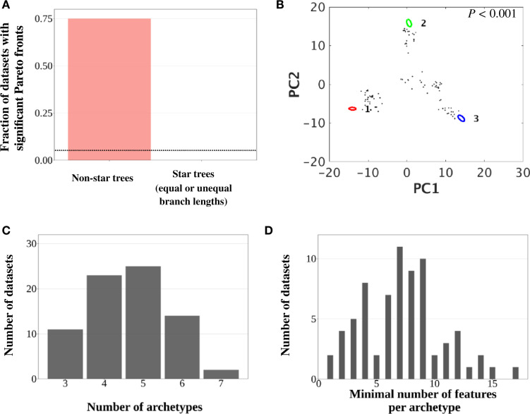
Phylogenetic relationships among study organisms cause false-positive identifications of Pareto fronts by ParTI. Simulated data with neutrally evolving phenotypes are used. (A) Fraction of data sets with statistically significant Pareto fronts. The dotted line shows the expected fraction in an unbiased test. (B) An example of the inferred Pareto front projected to the first two principal components of the phenotypic space. (C) Frequency distribution of the number of inferred archetypes among data sets with significant Pareto fronts. (D) Frequency distribution of the minimum number of uniquely enriched features per archetype in the 72 data sets with significant Pareto fronts and uniquely enriched features for every archetype.
As a control, we generated data sets without phylogenetic structures using star trees, because all taxa are phylogenetically equally distant from one another in a star tree. We first simulated the neutral evolution of 100 independent traits following a star tree of 100 species with equal branch lengths. We repeated this simulation 100 times, but no significant Pareto front was discovered (fig. 2A). The same was found when a star tree with unequal branch lengths was considered (fig. 2A).
Population Structures Cause False-Positive Errors
A population may contain multiple subpopulations such that mating within subpopulations is more likely than that between subpopulations. Such population structures could mislead ParTI in identifying spurious Pareto fronts from organisms of the same species. To verify this hypothesis, we simulated the neutral evolution of the genotypes of 1,000 individuals according to a population structure (Gutenkunst et al. 2009) resembling a simplified version of the human population with three subpopulations (fig. 3A) and then computed the phenotype of each individual from its genotype using an additive model (see Materials and Methods). The simulation was repeated 100 times.
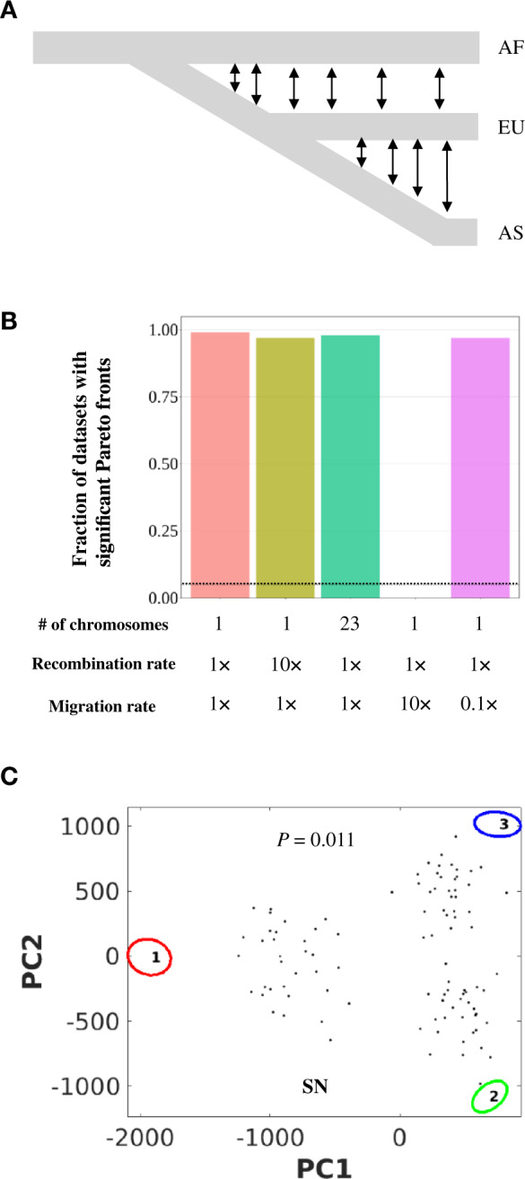
Population structure among study organisms cause false-positive identifications of Pareto fronts by ParTI. Simulated data with neutrally evolving phenotypes are used. (A) The out-of-Africa human demographic model is used in the simulation of neutral trait evolution. AF, African subpopulation; EU, European subpopulation; AS, Asian subpopulation. Double arrowheads indicate gene flows. (B) Fraction of data sets with statistically significant Pareto fronts. The dotted line shows the expected fraction in an unbiased test. The recombination and migrations rates indicated are relative to the base values provided in Materials and Methods. (C) An example of the inferred Pareto front projected to the first two principal components of the phenotypic space. The example is from the left-most bar of panel (B).
We found that ParTI inferred significant Pareto fronts with three archetypes more than 95% of the time despite that neutral evolution was simulated for the traits considered (left-most bar in fig. 3B). A typical example is shown in figure 3C. Furthermore, when using the subpopulation label (Africans, Europeans, and Asians) as discrete features in feature enrichment analysis, we found that in all cases, each archetype is enriched with one of the subpopulation labels, suggesting that the falsely identified archetypes reflect the subpopulations.
Because recombination between genotypes from different subpopulations reduces the population structure in the data, we assessed the impact of the recombination rate on our result. Interestingly, increasing the recombination rate to 10 times the human recombination rate does not substantially alter the ParTI result (second left bar in fig. 3B). Similarly, raising the effective recombination rate by breaking the single chromosome considered into 23 equal-size chromosomes does not qualitatively change the ParTI result (middle bar in fig. 3B). These observations are likely due to the low migration rates among subpopulations used in the simulation such that recombination primarily homogenizes genotypes within the same subpopulation. As expected, when we increased the migration rates among subpopulations by 10 fold, none of the 100 simulated data sets was found to be significantly Pareto optimal (second right bar in fig. 3B). Notwithstanding, in 39 of the 100 cases, each inferred archetype is significantly enriched with a different subpopulation, suggesting that the increased migration may not fully remove the population structure and that ParTI may still infer spurious Pareto fronts if the sample size is larger. On the contrary, when we reduced the migration rates to 10% of the original level, Pareto optimality was found to be significant at a frequency that is similar to that under the original migration rates (right-most bar in fig. 3B). Together, these findings reveal exceptionally frequent false-positive identifications of Pareto fronts by ParTI in the presence of population structure resembling that of humans.
The Flexibility of Data Analysis Inflates False Positives
In examining past studies that used ParTI and analyzing the real and simulated data, we noticed another potential source of false-positive errors—flexibility in data analysis, which provides an opportunity for p-hacking (Simmons et al. 2011). It has been well documented that the false-positive rate is substantially inflated when researchers are allowed to make many liberal decisions in data analysis (Simmons et al. 2011). The reason is simple: the probability that at least one of the many choices makes the result significant at the significance level of 0.05 is much higher than 0.05, the expected false-positive rate under a fixed procedure of data analysis.
Using ParTI to infer Pareto fronts and the associated tasks involves multiple steps, and the investigator has multiple decisions to make at each of these steps. As shown in figure 4A, to use ParTI, a researcher must first decide how to preprocess the data. Next, the researcher has to decide the number of potential archetypes by either using the default setting of ParTI (Hart et al. 2015) or manually specifying it (Hausser et al. 2019). In both cases, one has to first reduce the dimension of the data to a manually set number. Then, the researcher can choose one of five algorithms to compute Pareto fronts (Sisal, MVSA, MVES, SDVMM, and PCHA) (Hart et al. 2015). Among these five algorithms, Sisal, MVSA, and PCHA are most frequently used and have been claimed to show different advantages: Sisal is robust to outliers, MVSA is able to extract information from extreme points, and PCHA is stable with low iteration numbers (Hart et al. 2015). After the Pareto front is inferred, the researcher can perform feature enrichment analysis to infer the involved tasks. The features used can be any properties of the samples, discrete or continuous (Hart et al. 2015).
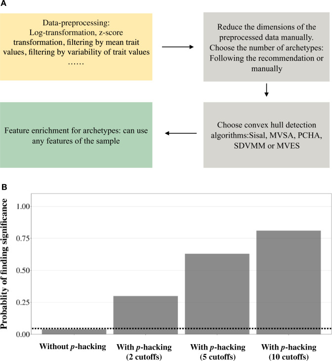
Flexibility in data analysis increases ParTI’s false-positive rate. (A) Pareto front inference involves multiple steps, each of which may be performed in multiple ways. (B) Fraction of data sets of neutral phenotypes that are detected by ParTI to have significant Pareto fronts. The number of ParTI analyses per raw data set equals four times the number of cutoffs considered (see Materials and Methods). The dotted line represents the expected fraction (5%) for an unbiased test.
Among the above steps, data preprocessing is probably the most flexible one. Let us take gene expression data preprocessing as an example. Starting from a raw data set, one may or may not normalize the data by the total expression level (Adler et al. 2019). Next, one can consider using log-transformation (Hart et al. 2015; Korem et al. 2015; Hausser et al. 2019), z-score transformation (Adler et al. 2019), or other transformations (Korem et al. 2015) to transform the data. Furthermore, one can filter the genes by their mean expression levels (Hart et al. 2015; Hausser et al. 2019) or the variability of gene expression levels typically measured by SD (Hart et al. 2015; Adler et al. 2019). Finally, one can decide to remove certain samples based on some flexible criteria. For example, the same breast cancer transcriptome data set used to detect Pareto fronts in cancer evolution was preprocessed differently in two studies; the normal tissue samples were retained in one study (Hart et al. 2015) but removed in the other (Hausser et al. 2019). To be fair to ParTI, most of the preprocessing techniques described above are also commonly used in other literature, especially in exploratory transcriptome analyses that are not associated with particular hypotheses. ParTI, however, is associated with a strong hypothesis that the phenotypes of the organisms examined have been optimized. As such, the flexibility in data analysis provides a huge space for p-hacking.
To illustrate this point, we simulated random phenotypes of 100 traits for each of 1,000 unrelated individuals and subjected the data to ParTI analysis (see Materials and Methods). Without data preprocessing, the false-positive rate of ParTI is 4% (fig. 4B). We then used various cutoffs to exclude genes from the analysis. For example, using the mean value cutoff of 20% excludes the 80% of traits with the lowest mean trait values, whereas using the SD cutoff of 20% excludes the 80% of traits with the lowest trait SDs. As the number of cutoffs explored in data preprocessing increases, the false-positive rate rises substantially (fig. 4B). When we explored 10 different cutoffs per data set (corresponding to 40 tests; see Materials and Methods), significant Pareto fronts were identified in 81% of the 100 replications (fig. 4B). Clearly, the flexibility in data preprocessing can cause a very high false-positive rate for ParTI. Note that the scenario considered here reflects a lower bound of the flexibility in data analysis because we only simulated part of the variations present in published ParTI studies (e.g., the variation in the number of archetypes specified was not simulated). With more researchers using ParTI, additional “creative” ways of data processing are expected.
Discussion
In this work, we investigated the false-positive rate of ParTI in testing Pareto optimality and identifying Pareto fronts. We discovered that, even when applied to a set of neutrally evolving or random traits, ParTI detects Pareto optimality with an extremely high probability, often reaching or exceeding 75%. In other words, the Type-I error of the method exceeds 0.75, whereas the expected value is 0.05 for an unbiased statistical test. These false-positive errors are attributable to either one of two sources. The first source is unequal relatedness among samples, such as the phylogenetic relationship and population structure among the organisms examined. This is a widespread problem in actual data, because it is difficult to find a large set of species that are all phylogenetically equally related with one another or a large group of phenotypically diverse conspecifics randomly sampled from a panmictic population. We did not explicitly study the influence of the pedigree structure of the examined individuals on the performance of ParTI, but the result is expected to be similar to those found under phylogenetic relationship and population structure, because all such scenarios involve unequal relatedness among samples. Even when individual cells from a multicellular organism are considered, because the cells are connected through a developmental cell lineage much like a phylogeny, somatic mutations or epigenetic changes will likely make the phenotypes of cells closer on the cell lineage more similar (Yang, Ruan, et al. 2014). Likewise, transcriptomes of single cells are often nonindependent due to spatial or temporal autocorrelation, which might create similar artifacts such as the horseshoe effect (Edelaar 2013; Hsu and Culhane 2020). Although we did not simulate the evolution of optimized traits, our results suggest that, even when the phenotypes are Pareto optimal, the Pareto front and archetypes identified by ParTI may be biased by the phylogenetic relationship or population structure in the data.
The second source of false-positive errors is the intrinsic flexibility of data preprocessing by ParTI. Because of the lack of a standard in data preprocessing, researchers are forced to explore their data in multiple ways; they may be tempted to continue exploring until the result fits their hypothesis even with no intention to p-hack. Note that we explored only a small set of data preprocessing techniques in this work. In reality, there are many more ways to preprocess data, especially for those phenotypes with no consensus methods of preprocessing. Our survey of past applications of ParTI shows that researchers often use additional post hoc adjustments. For instance, in the study of the mass-longevity Pareto front (Szekely et al. 2015), the authors “peeled” the data by removing data points on the inferred convex hull on the basis of the variation of the inferred archetype positions, and reported the new Pareto fronts after the peeling procedure. In another example, the beak morphologies of multiple individuals from each of six species of Darwin’s finches were analyzed for Pareto optimality (Shoval et al. 2012). It was pointed out that there are at most six independent data points here because phenotypes of the conspecifics are nonindependent; as a result, there is no statistical power for Pareto front identification (Edelaar 2013). However, the authors of ParTI adjusted the test to fit this data set—instead of shuffling the post-PCA dimension-reduced data, they shuffled the original data (Shoval et al. 2013). They found that the dimensionality of the randomly shuffled data is generally higher than that of the real data, measured by the fraction of variance unexplained by the first two PCs. Because the Pareto front is a low-dimensional shape in a high-dimensional space, they argued that this finding means that the Pareto front identified from only six independent data points is significant. But, by this standard, any biological data set with low dimensionality, which is virtually any biological data set because of the pervasive nonindependence among biological traits, will show a significant Pareto front.
It is important to stress that, in our study, we separately examined the impacts of the above two sources of error. In practice, the two sources are likely to be simultaneously present in a data set and its analysis. Hence, the actual false-positive rate is expected to be even higher than reported here. Our results thus raise substantial doubt about previous PartTI-based claims of Pareto optimality in biological data and the applicability of the idea of identifying Pareto fronts by fitting polytopes.
Are there other potential causes for ParTI’s false-positive errors in general? Biological data often have complex, nonrandom structures due to reasons unrelated to adaptation, such as the nonbiological clustering of the transcriptomes of single cells due to batch effects in performing the experiments (Hicks et al. 2018). Due to the difficulty in simulating data with these structures, we are unable to explore their impacts on ParTI. Nevertheless, because phylogenetic relationships and population structures simply mean a variation in phenotypic correlation among organisms, which could have many causes other than the evolutionary history (e.g., the batch effect or autocorrelation), ParTI is expected to be impacted by many factors unexplored here.
Although the causes of ParTI’s false-positive errors are clear for the simulated phenotypic data, what factors are responsible for ParTI’s error in analyzing the transcriptomes of yeast gene deletion strains? Because the gene deletion strains were all constructed from the same wild-type, the data have no phylogenetic relationship or population structure. Given that the technical replicate transcriptomes of the yeast wild-type strain also showed a significant Parent front and archetypes highly similar to those of the transcriptomes of gene deletion strains, the batch effect in performing the microarray experiments is likely to be at least one of the culprits. Additionally, we suspect that the flexibility in data preprocessing played a role, because the result became significant after we tried a couple of different preprocessing methods. Specifically, unlike typical microarray gene expression analysis, we did not use log-transformed expression levels in our analysis. Notwithstanding, we note that this way of analysis is acceptable (Gupta et al. 2006; Nguyen and Disteche 2006) and has even been used by the authors of ParTI (Adler et al. 2019) against their own advice in the ParTI manual of using log-transformed expressions (Hart et al. 2015). Our analysis of the transcriptome data from the yeast gene deletion strains illustrates the exact dilemma faced by researchers analyzing real data, because the dual functions of ParTI in data exploration and Pareto optimality testing make it difficult to decide how much data exploration is appropriate and when a significant test result is trustable.
Can the problems of ParTI discovered here be circumvented? We believe that it is possible to minimize the p-hacking problem by establishing a plan for data preprocessing before the analysis of the data (e.g., preregistration) and sticking to the plan in the analysis (Gonzales and Cunningham 2015; Nosek et al. 2018), although it may be difficult to determine a universal plan for all data sets given the huge heterogeneity of the type of data. The p-hacking problem is not unique to ParTI and solutions developed in other fields to this problem (Simmons et al. 2011) can be borrowed.
The problem caused by phylogenetic relationship or population structure in the data is more difficult to solve. This problem is almost unique to biology and permeates a large fraction of data sets that have been analyzed using ParTI (Shoval et al. 2012; Hart et al. 2015; Szekely et al. 2015; Tendler et al. 2015; Trink et al. 2018; Cona et al. 2019; Forkosh et al. 2019; Hausser et al. 2019). To the credit of the inventors of ParTI, two ad hoc solutions have been proposed to address the phylogenetic relationship problem. The first proposed solution is to show that trait distributions of species separated by a mass extinction fill the same polytope, under the premise that the species before and after a mass extinction would have different phylogenies so should not create the same polytope by phylogenetic relationships. This appears to be a valid argument, but it has very limited use, because phenotypic data of species separated by mass extinctions are rare. In fact, only one ParTI study could use and has used this approach (Tendler et al. 2015). The second proposed solution is to show that the phylogenetic relationship does not fully explain the polytope inferred. For example, in one study (Szekely et al. 2015), the authors explicitly noted that the phylogeny affects the inferred polytope. They then showed that 1) the correlation between phylogenetic distance and morphological distance is not perfect and 2) the positions of the species in the polytope are not fully concordant with those in the phylogeny. A similar argument was made in another ParTI study (Karin and Alon 2019). This type of argument for the validity of the identified Pareto fronts does not hold, because genetic drift or even measurement error could render the correlation/concordance imperfect. In other words, the observation that the correlation/concordance is imperfect does not rule out the influence of phylogenetic relationships nor establish optimization. Instead, the correct way to validate the identified Pareto fronts, which has never been done, is to demonstrate statistically that the remaining phenotypic variation after the control of phylogenic relationships is explained by Pareto optimality. In comparative biology and quantitative genetics, methods such as independent contrast (Felsenstein 1985) and variance component models (Kang et al. 2010) are available to deal with phylogenetic and population nonindependence, but it is not immediately clear how such methods can be applied to Pareto front identification in the context of fitting polytopes. One way to address this problem is to remove samples with phylogenetic or population structures from ParTI analysis. This would of course greatly diminish the utility of ParTI, because many fitness-related traits, such as body mass and life-history traits, are known to have strong phylogenetic signals (Kamilar and Cooper 2013). One can also remove traits that have strong phylogenetic signals based on some statistics such as Bloomberg’s K or Pagel’s (Münkemüller et al. 2012). Another solution might be a requirement that any claim of Pareto optimality must also be based on significant evidence for phenotypic selection, because phenotypes cannot be optimized without selection. However, this requirement does not alter the influence of phylogenetic and population structures on ParTI’s performance so does not remove the root of the problem. Furthermore, testing phenotypic selection itself is not a simple task. Finally, ParTI studies often use feature enrichment to guard against false positives, sometimes combined with computational or experimental validation of the enrichment. Similar to the process of interpreting Gene Ontology (GO) term enrichment (Brenner 2002), it is difficult to interpret enrichment results without ambiguity or circular reasoning. Furthermore, the validation confirms the enrichment, not Pareto optimality. Because our results showed that feature enrichment does not guard against false positives, the value of verifying feature enrichment for demonstrating Pareto optimality is minimal.
In summary, our results suggest that Pareto fronts cannot be reliably identified by fitting polytopes and that almost all ParTI-based Pareto fronts reported so far should be considered false until future validation by reliable methods. Notwithstanding, the difficulty in reliably identifying Pareto fronts from biological data does not imply that the concept of Pareto optimality or Pareto front is useless in biology. We believe that Pareto optimality is a valuable idea and hypotheses about Pareto optimality are worth testing. Very recently, Mikami and Iwasaki (2021) devised the flipping t-ratio test and showed that it can substantially reduce the false-positive rate of ParTI caused by phylogenetic structures in the data. When they applied this test to previously analyzed data where Pareto fronts were identified, including the beak morphologies of Darwin’s finches (Shoval et al. 2012), mammalian life-history traits (Szekely et al. 2015), and ammonite shell morphologies (Tendler et al. 2015), no significant Pareto fronts were found. As mentioned, the Pareto front inferred from the ammonite shell morphologies had been verified using a mass extinction, suggesting that even seemingly convincing verifications of ParTI results may not be immune to error. The flipping t-ratio test requires the knowledge of the phylogenetic tree of the organisms in the data and infers ancestral trait values at interior nodes of the tree. Although the development of this method is a large step forward toward reducing ParTI’s false-positive rate, the method is subject to the two common problems faced by comparative methods so is not errorproof. First, the true phylogenetic tree may not be known. Second, inferring ancestral states requires knowing the model of trait evolution, which is almost always unknown so has to be assumed. After all, if we knew the model, we would not need to use ParTI to test phenotypic optimization. Currently, it is unclear whether the flipping t-ratio test is sensitive to tree or model misspecification (Mikami and Iwasaki 2021). We thus call for further investigation of the flipping t-ratio test and further development of reliable methods in this area.
Materials and Methods
Preprocessing of the Transcriptomes of Yeast Gene Deletion Strains
From the website http://deleteome.holstegelab.nl/ (last accessed December 24, 2020) (Kemmeren et al. 2014), we downloaded the two-channel microarray gene expression data of 1,484 yeast gene deletion strains grown in the SC medium. Let mi be the expression level of gene i in a gene deletion strain, and wi be the expression level of the same gene in the wild-type. The data from each gene deletion strain contained the information of Mi and Ai for gene i defined below:
Therefore, , which provided the expression level estimates of gene i in the deletion strain as well as the wild-type. Because the expression levels measured here are meaningful only in a relative sense, we normalized the expression level of each gene in each strain by the sum of the expression levels of all genes in that strain. We retained the genes whose mean normalized expression levels are higher than 7.72 × 10⁻⁴, to strike a balance between the precision in the measurement of gene expression level and the number of genes that can be analyzed. Finally, we transformed the data into z-scores for each gene.
Some yeast gene deletion strains are fitter than the wild-type in the SC medium where the transcriptome data were collected, probably because of antagonistic fitness effects of genes across environments (Qian et al. 2012). To ensure that the transcriptomes used are nonoptimized, we also analyzed a subset of strains by excluding those gene deletion strains that are fitter than the wild-type in the SC medium, on the basis of published fitness of the gene deletion strains relative to the wild-type measured by barcode sequencing in SC (Qian et al. 2012).
To investigate whether Pareto fronts may be erroneously inferred from batch effects in quantifying the transcriptomes, we obtained the gene expression levels in all wild-type technical replicates by a similar procedure.
ParTI Analysis of the Transcriptomes of Yeast Gene Deletion Strains
Before analyzing the transcriptome data from the yeast gene deletion strains, we replicated several published results from ParTI analysis as well as examples in the ParTI package to ensure that we used ParTI as intended by its developers. Following the ParTI manual, we used the default “Sisal” algorithm to detect Pareto fronts from the preprocessed gene expression levels of the yeast gene deletion strains. The user-defined “dim” option, which specifies the number of PCs to retain in ParTI analysis, was set to 5 because the manual recommends it to be set between 5 and 10 (Hart et al. 2015). Similarly, the “binSize” option was set to 0.05 according to the manual (Hart et al. 2015). ParTI suggested three archetypes in the data, so the number of archetypes was set to 3. To perform the task inference, we used GO data from the GO2MSIG database (Powell 2014) (http://www.bioinformatics.org/go2msig/; last accessed December 24, 2020). We used all GO annotations, including IEA (GO terms inferred from electronic annotation). The genes were identified by the National Center for Biotechnology Information gene IDs. We similarly analyzed the gene deletion strains less fit than the wild-type and the wild-type replicates, respectively. We fixed the number of archetypes to 3 when analyzing these two data sets.
Simulation of Neutral Trait Evolution along Phylogenies and the Subsequent ParTI Analysis
We first generated phylogenetic trees with 100 tips using a birth–death process with the birth rate being 1 per unit time and the death rate being a uniform random variable sampled between 0 and 1 per unit time. We then simulated the neutral evolution of 100 independent traits according to the standard Brownian motion model (Harmon 2018). The rate of the Brownian motion was set at 1 per unit time for every trait, meaning that, starting from a mean trait value of μ, the mean trait value after t units of time of evolution is a normal random value with the mean equal to μ and variance equal to t. The simulation of trait evolution was performed using the “sim.traits” function in the “phylocurve” package (Goolsby 2015). For comparison, we simulated the neutral evolution of traits without phylogenetic relations (i.e., along a star phylogeny with equal branch lengths) (Harmon 2018). To achieve this goal, we used Pagel’s λ transformation, which stretches external branches of a tree relative to the internal branches, and set λ at 0. We also simulated neutral evolution along a star phylogeny with unequal branch lengths by randomly sampling the 100 branch lengths from a uniform distribution between 0 and 1 unit time and simulating trait evolution along these branches.
To simulate the evolution of 100 independent binary traits, we used the “sim.char” function in the “phylocurve” package. For each trait, the rate parameters were specified by the following Q matrix of the Markov process: .
We repeated the above process 100 times to generate 100 trees (the death rate varies among trees), each associated with a data set of 100 species, each having 100 continuous traits and, when the identified Pareto front is statistically significant, 100 additional binary traits.
We followed the ParTI manual to infer Pareto fronts and the associated tasks from the simulated data sets. The algorithm used was “Sisal.” The “dim” option was set to 8, which is in the middle of the manual-recommended range of [5, 10]; use of other dim values did not qualitatively alter the result. The “binSize” option was set to 0.2. We let ParTI automatically determine the number of archetypes in each data set.
Simulation of Neutral Trait Evolution According to a Human Demographic Model and the Subsequent ParTI Analysis
We used “msprime” (Kelleher et al. 2016) to generate the neutrally evolved genotypes of 100 diploid individuals. Limited by the amount of computational time required, we simulated only one of the 23 human chromosomes. The basic parameters were set according to a published population structure model describing the out-of-Africa origin of human populations with three main subpopulations—Africans, Europeans, and Asians—subject to intersubpopulation gene flow (Gutenkunst et al. 2009). We sampled 33 Africans (by randomly pairing 66 haplotypes sampled from the African subpopulation), 33 Europeans, and 34 Asians. We set the chromosome size to 108 bases, roughly the size of an average human chromosome. The mutation rate was set to 10−8 per base per generation, and the recombination rate was set to 10−8 per base per generation, corresponding to the known parameters for humans (Milo et al. 2010). The above process was repeated 100 times to generate 100 independent data sets.
To assess the impact of recombination rate on our result, we generated 100 additional data sets with a recombination rate of 10−7 per base per generation. In addition, we generated 100 data sets by breaking the single chromosome into 23 chromosomes of 108/23 bases to add random assortment. To assess the impact of the migration rate on our result, we generated 100 data sets with 10 times the original migration rates and another 100 data sets with 10% of the original migration rates.
After simulating the genotype of each individual, we generated the trait values for 100 traits from the genotype. In the simulation, every locus has two alleles in the population, specified by 0 and 1, respectively. The effect of allele 0 on any trait is 0, and the effect of allele 1 on a trait is a standard normal random variable. The trait value will be the sum of effects from all loci on the trait. This simulation is consistent with the universal pleiotropy model in which every locus affects every trait (Wagner and Zhang 2011). The simulated phenotypes were then analyzed by ParTI with default settings to detect three archetypes. The population labels of the output samples were supplied as features to perform the feature enrichment analysis.
Simulation of p-Hacking
To illustrate the point that flexibility in data analysis can lead to p-hacking, we simulated the phenotypes of 100 traits for 1,000 individuals. In each individual, the trait values were sampled from a multivariate normal distribution specified by a 100-dimension vector, whose entries are uniform random variables between 1 and 10 representing the mean phenotypic values of the 100 traits, and a 100 × 100 variance–covariance matrix. The variance–covariance matrix was based on a random trait–trait correlation matrix generated by the program “genPositiveDefMat” from the package “clusterGeneration” with default setting (Joe 2006), coupled with the variance of each trait generated by a random draw from the uniform distribution between 1 and 10. From this raw random phenotypic data set, we generated 40 data sets by commonly used preprocessing techniques. That is, we retained traits among the highest 10%, 20%, …, and 100% of traits in terms of the mean trait value or in terms of the SD, resulting in 20 data sets. From each of these 20 data sets, we converted the trait values to z-scores across individuals, generating 20 additional data sets. We then mimicked three different levels of p-hacking by considering two (50% and 100%), five (20%, 40%, 60%, 80%, and 100%), and all 10 cutoffs in terms of the mean trait value or SD, corresponding to 8, 20, and 40 ParTI analyses per raw data set, respectively. The algorithm used in the ParTI analysis was “PCHA,” another algorithm that was widely used in past ParTI studies. Because the raw phenotypic data are completely random, all Pareto fronts identified are false positives. To restrict the flexibility of ParTI in Pareto front inference, we fixed the number of archetypes to 3 by setting the variable “ForceNArchetypes” in ParTI to 3. The above data generation, preprocessing, and ParTI analysis were repeated 100 times.
Acknowledgments
We thank Tomoyuki Mikami and Wataru Iwasaki for sharing their manuscript before publication and members of the Zhang lab, Pim Edelaar, and an anonymous reviewer for valuable comments. This work was supported in part by U.S. National Institutes of Health research grant GM103232 to J.Z.
Data Availability
There are no data to be archived. Computer code and intermediate results are available at https://github.com/mengysun/False_positive_ParTi.