Introduction

Electronegativity is defined as the tendency of an atom to attract electron density, i.e., to polarize the chemical bond. The concept of electronegativity can be traced back to 1819 when great Jöns Jacob Berzelius divided the elements into electropositive and electronegative¹. This was already useful, even as a qualitative concept that arrived well before the discovery of the electron in 1897². Then, in 1916, Gilbert Newton Lewis formulated his theory of chemical bonding, according to which chemical bond is a result of sharing valence electrons.³ Development of this theory has led Linus Pauling to formulate in 1932 a quantitative concept of electronegativity (X) based on thermochemistry⁴. Pauling derived values of X from bond energies, assuming that extra stabilization of a bond due to its polarization is an additive effect, expressed in electron-volts as

Furthermore, tabulated values of Pauling’s electronegativity for many elements are strange: for example, electronegativities of such metals as Ru, Rh, Pd, Os, Ir, Pt, Au, W, and Mo are higher than the values for B and H, which would imply a positive charge on boron and negative charge on those metal atoms in their borides or hydrides– this is completely counterintuitive. One can also notice a strange dimensionality of Pauling’s electronegativities, eV^1/2.

Spectroscopic scales of electronegativity are based on data on isolated atoms, among them the Mulliken^9,10, Allen^11–13, Martynov and Batsanov¹⁴, and many other scales. Mulliken electronegativity^9,10 is defined as the average of the ionization potential and electron affinity. This gives an absolute scale, where electronegativities have a meaningful dimensionality (eV) and have the physical meaning of minus the chemical potential of the electron in an atom, as supported by density functional theory^15–19, which reinforced the position of Mulliken’s definition. Charge transfer from the less electronegative atom to the more electronegative one can then be viewed as a consequence of equalization of their chemical potentials. The beauty of this scale is counterweighted by difficulties of obtaining electron affinities, which for many elements are still not well known.

Allen^11–13 proposed another popular spectroscopic scale, where electronegativity is equal to the average energy of valence electrons in a free atom. This approach suffers from an ambiguity as to which electrons should be considered as valence for d- and f-elements. Martynov & Batsanov¹⁴ used the square root of the average valence ionization energy as a measure of electronegativity, and their electronegativities have the same dimensionality as Pauling’s, i.e., eV^1/2. Martynov–Batsanov values are very close to Pauling’s, highlighting that completely different definitions converge on the same truth.

Here we reevaluate the concept of electronegativity, which is a key property of the elements expressed many years ago. We identify the drawbacks in the definition of Pauling’s electronegativity scale and reformulate our thermochemical scale on experimental dissociation energies. Our scale displays intuitively correct trends for the 118 elements across the periodic table and reasonably predicts the degrees of ionicity of chemical bonds, improves the separation of elements into metals and non-metals, and greatly improves the description of thermochemistry of molecules and chemical reactions.

Results and discussion

Let us come back to formula (1) and try to apply it. One can expect the results to be most accurate (greatest signal/noise ratio) at large $$ \mathrm{\Delta }{X}_{\mathrm{AB}}^2$$, so we start with alkali and alkali earth fluorides. From experimental bond dissociation energies^20–59 we find that the ionic stabilization energy is greater in LiF than in CsF or in any alkali fluoride. According to (1) this should indicate that Li is the most electropositive alkali metal and overall electronegativity increases down the group of the periodic table—which is exactly contrary to chemical intuition and to the values one finds in Pauling’s scale. Strangely, Pauling’s electronegativities of alkali metals (and, equally badly, alkali earth metals) cannot be obtained from their highly ionic molecules using Pauling’s formula (1). The values one finds from (1) and experimental bond dissociation energies are X(Li) = 1.85, X(Na) = 1.96, X(K) = 1.99, X(Rb) = 2.00, X(Cs) = 1.93; these are very different from standard Pauling’s electronegativities of 0.98, 0.93, 0.82., 0.82, and 0.79, respectively (see Supplementary Fig. 1).

The problem is in the form of formula (1): Li–F bond length is much shorter than Cs–F and ionic term should of course be stronger in the shorter bond in Li⁺F⁻ than in Cs⁺F⁻. The same is true for the covalent part of the bond energy, which is also greater in LiF than in CsF. Ionic effects are larger in CsF than in LiF only in relative (relative to covalent effects), but not in absolute sense (see Table 1). This leads to ionic stabilization being not an absolute additive term, but a multiplicative enhancement factor, and the simplest formula is

Table 1

Bond energetics for alkali fluorides.

Molecule	Dissociation energy $$ D_{\mathrm{AB}}$$, eV	Covalent part $$ D_{\mathrm{AB}}^{\mathrm{cov}}$$, eV	Ionic part $$ D_{\mathrm{AB}}^{\mathrm{ion}}=D_{\mathrm{AB}}-D_{\mathrm{AB}}^{\mathrm{cov}}$$, eV
Li–F	6.001	1.380	4.621
Na–F	5.379	1.220	4.159
K–F	5.127	1.086	4.041
Rb–F	5.091	1.074	4.017
Cs–F	5.327	1.039	4.288

Now, electronegativities as defined by formula (2) are dimensionless (see Fig. 1). With the help of formula (2) we recover correct trends for the whole periodic table, and do not encounter pathologies such as those mentioned above for alkali and alkali earth metals. All metals have lower electronegativities than boron and hydrogen—in better agreement with chemical intuition than Pauling’s values. Applying formula (2) to molecules ClF, BrF, IF, we obtained electronegativities of Cl (3.56), Br (3.45), I (3.22). Then we recalculated electronegativities of alkali metals using alkali chloride, bromide, and iodide molecules, and found the same values within ~0.2 (which can be considered as uncertainty of our values): for example, the electronegativity of Na extracted from NaF is 2.15, from NaCl 2.28, from NaBr 2.13, from NaI 1.94. Electronegativities of all 118 known elements were calculated using experimental dissociation energies^20–59 (we took averages of the reported values when two or more measurements were available, see Supplementary Table 2) and are shown in Fig.1. Electronegativities of some elements where there are not enough reliable data on bond energies (noble gases, Pm, Ra, Po, At, and some of the heaviest elements) were obtained indirectly, via a linear correlation with their experimental Mulliken electronegativities, because Mulliken scale shows the best correlation with our scale. In fact, our thermochemical scale has reasonable linear correlation with all other scales (Fig. 2 and Supplementary Table 3), Pearson correlation coefficient R being 98% for Mulliken and Allen scales, 87% for Pauling, and 85% for Martynov–Batsanov scales). For short-lived 6d- and 7p-elements Rf, Db, Sg, Bh, Hs, Mt, Ds, Rg, Cn, Nh, Fl, Mc, Lv, Ts, Og we obtained thermochemical electronegativities from theoretical Mulliken electronegativities^60,61. When more data become available for these elements, then thermochemical electronegativities will be determined directly. Interestingly, the slope of the correlation line is 1/2 for Pauling’s and Martynov–Batsanov scales, 2/3 for Allen’s and 1/4 for Mulliken’s scale. One can see the expected trends in the periodic table: periodicity of electronegativities, and their overall decrease from top to bottom of the table. The highest electronegativities are those of halogens and noble gases; the lowest—of alkali metals (Li: 2.17, Cs: 1.97) and, surprisingly, some other metals (Zr: 2.05, Hf: 2.01, and two anomalous lanthanoids are even slightly lower than Cs–Eu: 1.81, Yb: 1.78). For the non-alkali anomalous metals, low values are consistent with their tendency to react highly exothermically with oxygen and fluorine; Yb even vigorously reacts with water. It is also known that Eu and Yb (and to a lesser extent Sm) display chemical behavior which is different from the other lanthanoids, preferring divalent state. From the viewpoint of physical properties, Yb has more than two times higher electrical conductivity than the other lanthanoids, and both Eu and Yb have work functions which are lower than those of the other lanthanoids and among the lowest in the periodic table (2.5 and 2.6 eV, respectively—compared with 2.9 eV for Li, 2.36 eV for Na, and 3.5 eV for La⁶²).

Fig. 1

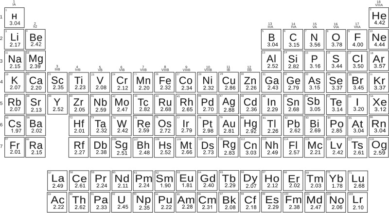
Periodic Table of our thermochemical electronegativities.

Electronegativities were obtained using the formula $$ D_{\mathrm{AB}}=D_{\mathrm{AB}}^{\mathrm{cov}}\cdot \left(1+\mathrm{\Delta }{X}_{\mathrm{AB}}^2\right)$$ (see Eq. 2), where $$ D_{\mathrm{AB}}$$ is the dissociation energy of chemical bond between two different atoms A and B, $$ D_{\mathrm{AB}}^{\mathrm{cov}}$$ is the covalent dissociation energy modeled as the arithmetic mean of the homonuclear dissociation energies and $$ \mathrm{\Delta }{X}_{\mathrm{AB}}^2$$ is the square of thermochemical electronegative difference between atoms A and B. The electronegativity values of the elements are also provided as Supplementary Data 1.

Fig. 2

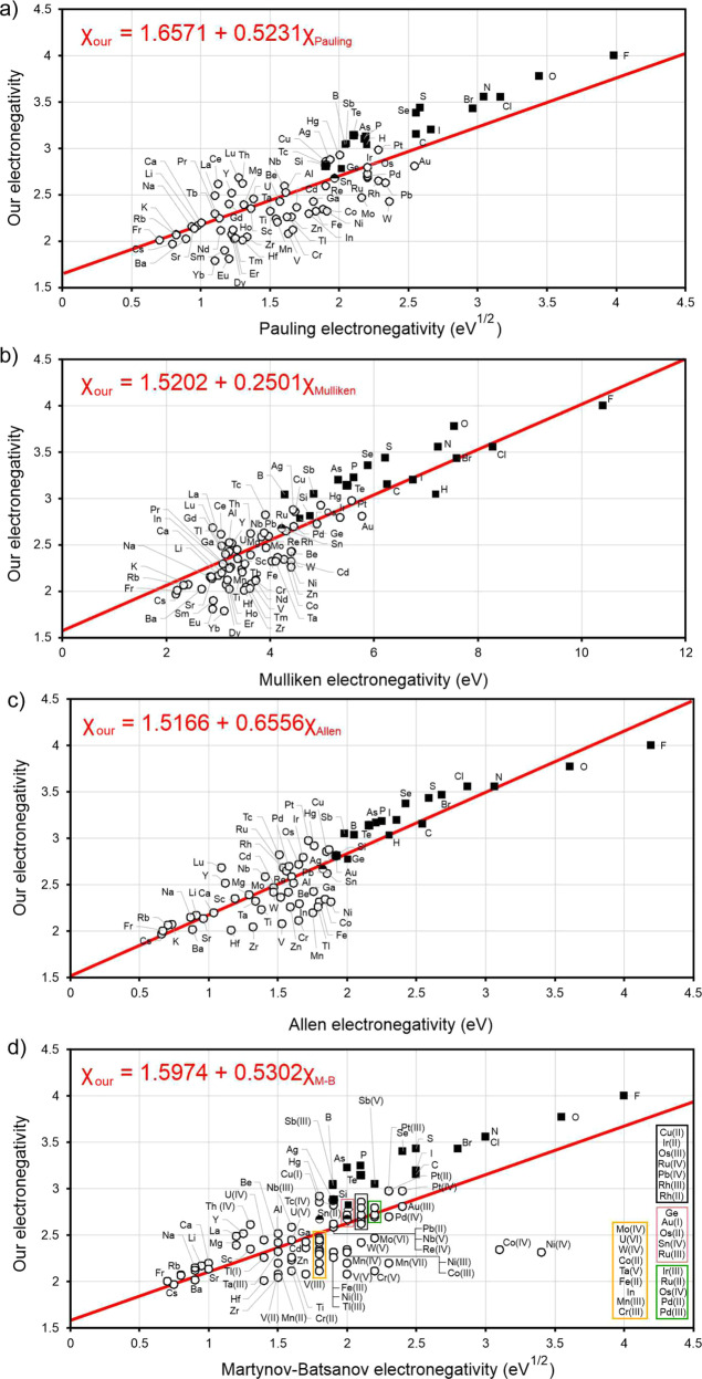
The correlation between our thermochemical electronegativities (X_our) on y-axis (dimensionless) with others electronegativities (x-axis).

(a) X_our vs Pauling (in eV^1/2), (b) X_our vs Mulliken (in eV), (c) X_our vs Allen (in eV), and (d) X_our vs Martynov-Batsanov (in eV^1/2). Lines indicate the linear correlation. Legend: metals, empty circles; non-metals, full square.

Electronegativity can be used as a criterion to discriminate between metals and non-metals, but different scales do so with different degrees of success. The best separation into metals and non-metals is achieved with our and Allen’s scales. For example, all elements with electronegativity above 3 (in our scale) are non-metals. Almost all elements with electronegativity below 3 are metals; the few exceptions are Si (2.82), Ge (2.79), Sn (2.68, but Sn is known at normal conditions in the metallic white tin and semiconducting gray tin allotropes). The scales of Pauling, Mulliken and Martynov–Batsanov work well too, but have difficulties assigning noble metals and a few other elements. From our table of electronegativities (Fig. 1), one can expect oganesson (Og, element #118, belonging to the group of noble gases) to be much more reactive than noble gases: with electronegativity as low as 2.59, it is expected to be a metal similar to Pb (electronegativity 2.62). Such low electronegativity comes from relativistic effects, which are particularly strong in superheavy elements, and non-inertness of Og is consistent with suggestions from literature^63–65. By contrast, due to relativistic stabilization of its valence 7s² shell, copernicium (Cn, element #112), belonging to the same group as mercury, has an anomalously high electronegativity of 3.03, similar to radon (electronegativity 3.04), non-metallic and rather inert element. Due to relativistic effects, some superheavy elements display unexpected similarity to other groups of the periodic table^66,67.

Pauling⁴ argued that extra stabilization of a bond (see formulae (1) and (2)) is due to a resonance mixing of covalent and ionic wavefunctions, the resulting charge asymmetry being determined by electronegativity difference. Pauling proposed to estimate the degree of ionicity by the heuristic formula:

Fig. 3

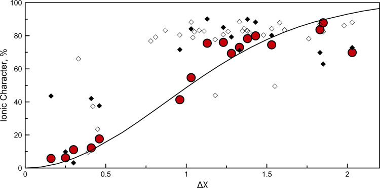
Ionic character in diatomic molecules.

Bond ionic character (IC) for different compounds calculated from dipole moment (i.e., red circles) and Bader charges for molecules (i.e., filled diamonds) and crystals (i.e., open diamonds) vs electronegativity difference (our scale).

We see that our electronegativity scale leads to correct bond polarity even where Pauling’s scale fails. For example, Pauling electronegativities of Ru, Rh, Pd, Os, Ir, Pt, Au, W, and Mo are higher than those of H and B, and one would obtain negative charges on metal atoms in their borides and hydrides. In our scale the opposite is the case, which agrees with the calculated Bader charges: e.g., W^+0.69 B^−0.69, Mo^+0.61 B^−0.61, Au^+0.14 B₂^−0.07, Pt^+0.24 H₄^−0.06.

There is some physical difference between our use of function (4) and Pauling’s. In our case, the squared electronegativity difference in the exponent in (4) is the ratio of the ionic and covalent contributions to bond energy. This should be more directly related to the degree of ionicity than just the ionic contribution taken without regard for the covalent energy (as in Pauling’s version).

Derived from thermochemistry, our electronegativity scale should be capable of at least qualitatively correctly predicting the outcome of chemical reactions, heats of formation and atomization energies of molecules and solids. To correct deficiencies of Pauling’s formula (1), Matcha⁸ introduced another formula (with energies in eV):

Fig. 4

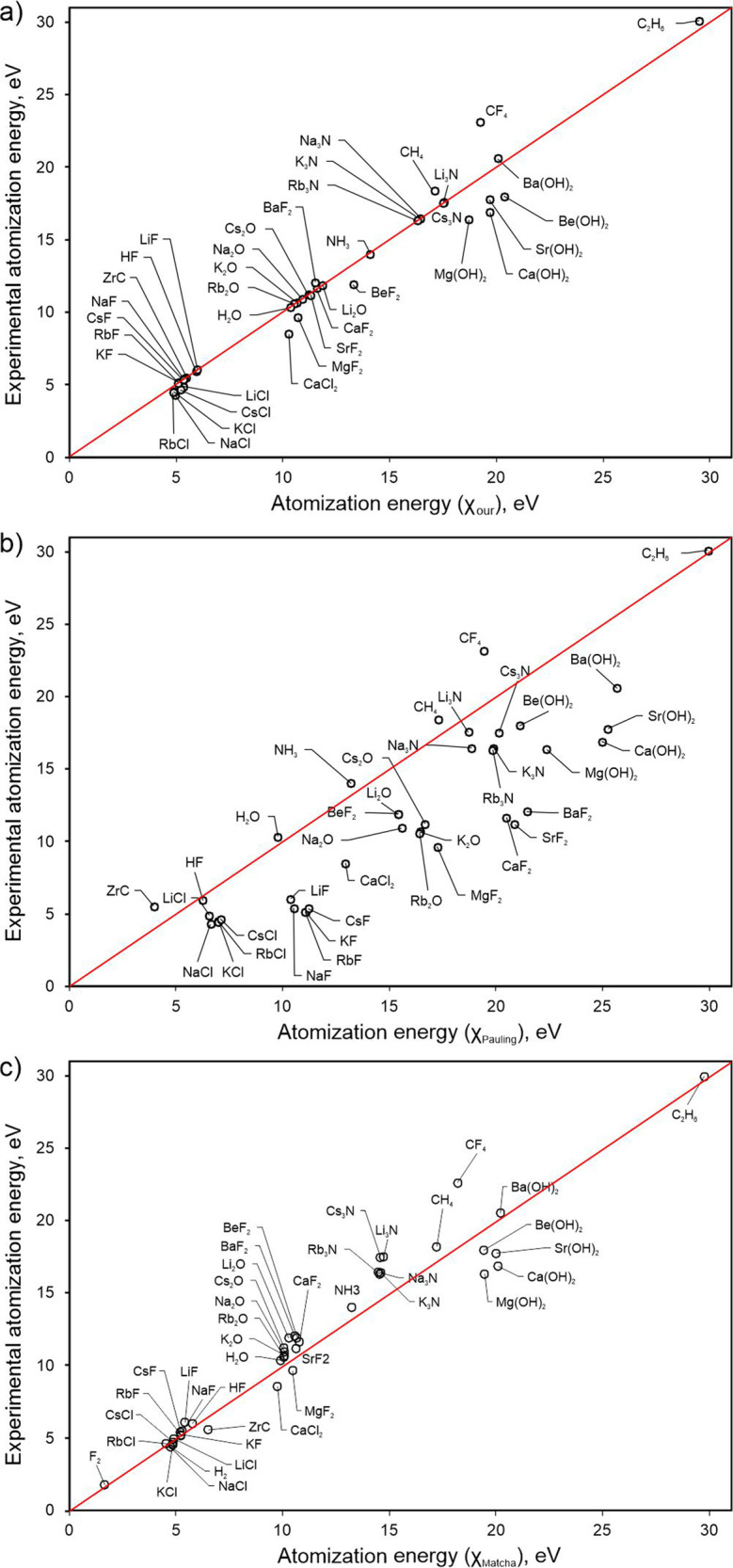
Atomization energies predicted from thermochemical electronegativities (x-axis) for a number of simple molecules in comparison with experimental atomization energies on y-axis.

(a) Experimental vs our, (b) experimental vs Pauling’s (c) and experimental vs Pauling’s corrected by Matcha ⁸. Lines indicate the ideal results, the root-mean-square deviations from which are 0.17 eV/atom for our approach, 1.21 eV/atom for Pauling’s, and 0.25 eV/atom for Matcha’s (the relative errors on atomization energies are 5%, 40, and 7%, respectively).

The same approach can be used for estimating the enthalpies of the formation of compounds. Taking the NaCl molecule again as example, we predict the energy of the reaction of its formation in the gas phase (Na₂ + Cl₂ = 2NaCl) as −6.31 eV using our electronegativity scale, and as −9.85 eV from Pauling’s approach and −9.42 eV from Matcha’s approach; clearly, the estimation based on our electronegativities is much closer to experiment (−5.27 eV from experimental energies of molecules⁵⁹). Large negative value indicates that the formation of NaCl from the elements is highly favorable.

Thermochemical electronegativities should be capable of predicting the direction of at least simple chemical reactions. It is known that Pauling’s electronegativities often lead to incorrect predictions¹². Let us take the reaction:

Ignoring the ionic term, one would find that the enthalpy of this reaction is zero. Pauling’s electronegativities and formula (1) give a positive value, +0.23 eV, incorrectly predicting that this reaction is unfavorable. Matcha’s approach gives +0.11 eV. Our electronegativity scale and formula (2) show that this molecular reaction is favorable, with enthalpy −0.45 eV. The experimental value is −0.92 eV⁵⁹. Figure 5 shows energies of very different exchange reactions (from reaction (3) to hydrolysis of Li₃N and fluorination of methane) calculated using electronegativities and using experimental molecular energies. One can see that in virtually all cases our model predicts the correct sign and reasonable magnitude of the reaction energy, in contrast to predictions based on Pauling’s approach. Our approach is also clearly much more accurate than Matcha’s.

Fig. 5

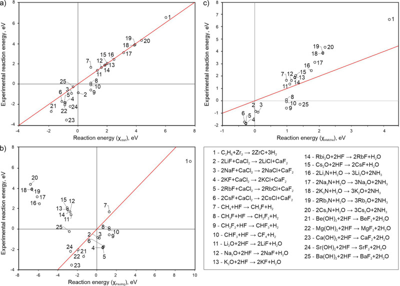
Comparison between predicted energies of 25 exchange reactions from thermochemical electronegativities (x-axis) and and experimental energies on y-axis.

(a) Experimental vs our, (b) experimental vs Pauling’s (c) and experimental vs Pauling’s corrected by Matcha ⁸. Lines indicate the ideal result (the root-mean-square deviations are equal to 0.9 eV for our approach, 5.1 eV for Pauling’s and 1.9 eV for Matcha’s).

Electronegativity is expected to correlate with many physical properties of materials—from mechanical (such as hardness, see—Ref. ^69,70) to electronic, optical etc. We showed above how well it discriminates between metals and non-metals. It can be expected to correlate with the work function, which (just like Mulliken’s electronegativity for an isolated atom) is equal to the chemical potential of the electron on the surface. This link has been known before^71,72, although the correlation is not perfect (see Supplementary Fig. 7): the best correlation coefficient (91%) is for Pauling’s scale, followed by Mulliken’s (83%), Martynov-Batsanov (79%), our (65%) and Allen’s (63%) scales, because o effects of the crystal structure (which lead to broadening of valence electron energy levels) and of the surface (the work function varies significantly between different surfaces of the same material).

To sum up, we have shown how a simple modification of the definition of thermochemical electronegativity leads to a greatly improved electronegativity scale. Our electronegativities are dimensionless (instead of unusual units eV^1/2 of Pauling’s electronegativities), display intuitively correct trends across the periodic table, allow for reasonable prediction of bond polarity and degree of ionicity, improve the separation of elements into metals and non-metals, and, most importantly, greatly improve the description of thermochemistry of molecules and chemical reactions. We expect our scale of electronegativity to find widespread use in chemistry and physics.

Methods