
Variational quantum algorithms (VQAs) optimize the parameters θ of a parametrized quantum circuit V(θ) to minimize a cost function C. While VQAs may enable practical applications of noisy quantum computers, they are nevertheless heuristic methods with unproven scaling. Here, we rigorously prove two results, assuming V(θ) is an alternating layered ansatz composed of blocks forming local 2-designs. Our first result states that defining C in terms of global observables leads to exponentially vanishing gradients (i.e., barren plateaus) even when V(θ) is shallow. Hence, several VQAs in the literature must revise their proposed costs. On the other hand, our second result states that defining C with local observables leads to at worst a polynomially vanishing gradient, so long as the depth of V(θ) is O(logn)
Parametrised quantum circuits are a promising hybrid classical-quantum approach, but rigorous results on their effective capabilities are rare. Here, the authors explore the feasibility of training depending on the type of cost functions, showing that local ones are less prone to the barren plateau problem.
One of the most important technological questions is whether Noisy Intermediate-Scale Quantum (NISQ) computers will have practical applications1. NISQ devices are limited both in qubit count and in gate fidelity, hence preventing the use of quantum error correction.
The leading strategy to make use of these devices is variational quantum algorithms (VQAs)2. VQAs employ a quantum computer to efficiently evaluate a cost function C, while a classical optimizer trains the parameters θ of a Parametrized Quantum Circuit (PQC) V(θ). The benefits of VQAs are three-fold. First, VQAs allow for task-oriented programming of quantum computers, which is important since designing quantum algorithms is non-intuitive. Second, VQAs make up for small qubit counts by leveraging classical computational power. Third, pushing complexity onto classical computers, while only running short-depth quantum circuits, is an effective strategy for error mitigation on NISQ devices.
There are very few rigorous scaling results for VQAs (with exception of one-layer approximate optimization3–5). Ideally, in order to reduce gate overhead that arises when implementing on quantum hardware one would like to employ a hardware-efficient ansatz6 for V(θ). As recent large-scale implementations for chemistry7 and optimization8 applications have shown, this ansatz leads to smaller errors due to hardware noise. However, one of the few known scaling results is that deep versions of randomly initialized hardware-efficient ansatzes lead to exponentially vanishing gradients9. Very little is known about the scaling of the gradient in such ansatzes for shallow depths, and it would be especially useful to have a converse bound that guarantees non-exponentially vanishing gradients for certain depths. This motivates our work, where we rigorously investigate the gradient scaling of VQAs as a function of the circuit depth.
The other motivation for our work is the recent explosion in the number of proposed VQAs. The Variational Quantum Eigensolver (VQE) is the most famous VQA. It aims to prepare the ground state of a given Hamiltonian H = ∑αcασα, with H expanded as a sum of local Pauli operators10. In VQE, the cost function is obviously the energy of the trial state . However, VQAs have been proposed for other applications, like quantum data compression11, quantum error correction12, quantum metrology13, quantum compiling14–17, quantum state diagonalization18,19, quantum simulation20–23, fidelity estimation24, unsampling25, consistent histories26, and linear systems27–29. For these applications, the choice of C is less obvious. Put another way, if one reformulates these VQAs as ground-state problems (which can be done in many cases), the choice of Hamiltonian H is less intuitive. This is because many of these applications are abstract, rather than associated with a physical Hamiltonian.
We remark that polynomially vanishing gradients imply that the number of shots needed to estimate the gradient should grow as . In contrast, exponentially vanishing gradients (i.e., barren plateaus) imply that derivative-based optimization will have exponential scaling30, and this scaling can also apply to derivative-free optimization31. Assuming a polynomial number of shots per optimization step, one will be able to resolve against finite sampling noise and train the parameters if the gradients vanish polynomially. Hence, we employ the term “trainable” for polynomially vanishing gradients.
In this work, we connect the trainability of VQAs to the choice of C. For the abstract applications in refs. 11–29, it is important for C to be operational, so that small values of C imply that the task is almost accomplished. Consider an example of state preparation, where the goal is to find a gate sequence that prepares a target state . A natural cost function is the square of the trace distance DT between and , given by , which is equivalent to
However, here we argue that this cost function and others like it exhibit exponentially vanishing gradients. Namely, we consider global cost functions, where one directly compares states or operators living in exponentially large Hilbert spaces (e.g., and ). These are precisely the cost functions that have operational meanings for tasks of interest, including all tasks in refs. 11–29. Hence, our results imply that a non-trivial subset of these references will need to revise their choice of C.
Interestingly, we demonstrate vanishing gradients for shallow PQCs. This is in contrast to McClean et al.9, who showed vanishing gradients for deep PQCs. They noted that randomly initializing θ for a V(θ) that forms a 2-design leads to a barren plateau, i.e., with the gradient vanishing exponentially in the number of qubits, n. Their work implied that researchers must develop either clever parameter initialization strategies32,33 or clever PQCs ansatzes4,34,35. Similarly, our work implies that researchers must carefully weigh the balance between trainability and operational relevance when choosing C.
While our work is for general VQAs, barren plateaus for global cost functions were noted for specific VQAs and for a very specific tensor-product example by our research group14,18, and more recently in29. This motivated the proposal of local cost functions14,16,18,22,25–27, where one compares objects (states or operators) with respect to each individual qubit, rather than in a global sense, and therein it was shown that these local cost functions have indirect operational meaning.
Our second result is that these local cost functions have gradients that vanish polynomially rather than exponentially in n, and hence have the potential to be trained. This holds for V(θ) with depth . Figure 1 summarizes our two main results.

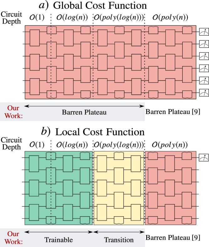
Summary of our main results.
McClean et al.9 proved that a barren plateau can occur when the depth D of a hardware-efficient ansatz is . Here we extend these results by providing bounds for the variance of the gradient of global and local cost functions as a function of D. In particular, we find that the barren plateau phenomenon is cost-function dependent. a For global cost functions (e.g., Eq. (1)), the landscape will exhibit a barren plateau essentially for all depths D. b For local cost functions (e.g., Eq. (2)), the gradient vanishes at worst polynomially and hence is trainable when , while barren plateaus occur for , and between these two regions the gradient transitions from polynomial to exponential decay.
Finally, we illustrate our main results for an important example: quantum autoencoders11. Our large-scale numerics show that the global cost function proposed in11 has a barren plateau. On the other hand, we propose a novel local cost function that is trainable, hence making quantum autoencoders a scalable application.
To illustrate cost-function-dependent barren plateaus, we first consider a toy problem corresponding to the state preparation problem in the Introduction with the target state being . We assume a tensor-product ansatz of the form , with the goal of finding the angles θj such that . Employing the global cost of (1) results in . The barren plateau can be detected via the variance of its gradient: , which is exponentially vanishing in n. Since the mean value is , the gradient concentrates exponentially around zero.
On the other hand, consider a local cost function:
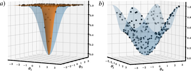
Cost function landscapes.
a Two-dimensional cross-section through the landscape of for n = 4 (blue) and n = 24 (orange). b The same cross-section through the landscape of is independent of n. In both cases, 200 Haar distributed points are shown, with very few (most) of these points lying in the valley containing the global minimum of CG (CL).
Moreover, this example allows us to delve deeper into the cost landscape to see a phenomenon that we refer to as a narrow gorge. While a barren plateau is associated with a flat landscape, a narrow gorge refers to the steepness of the valley that contains the global minimum. This phenomenon is illustrated in Fig. 2, where each dot corresponds to cost values obtained from randomly selected parameters θ. For CG we see that very few dots fall inside the narrow gorge, while for CL the narrow gorge is not present. Note that the narrow gorge makes it harder to train CG since the learning rate of descent-based optimization algorithms must be exponentially small in order not to overstep the narrow gorge. The following proposition (proved in the Supplementary Note 2) formalizes the narrow gorge for CG and its absence for CL by characterizing the dependence on n of the probability C ⩽ δ. This probability is associated with the parameter space volume that leads to C ⩽ δ.
Let θj be uniformly distributed on [−π, π] ∀j. For any δ ∈ (0, 1), the probability that CG ≤ δ satisfies
For our general results, we consider a family of cost functions that can be expressed as the expectation value of an operator O as follows
It is typical to express O as a linear combination of the form . Here Oi ≠ , , and we assume that at least one ci ≠ 0. Note that CG and CL in (1) and (2) fall under this framework. In our main results below, we will consider two different choices of O that respectively capture our general notions of global and local cost functions and also generalize the aforementioned CG and CL.
As shown in Fig. 3a, V(θ) consists of L layers of m-qubit unitaries Wkl(θkl), or blocks, acting on alternating groups of m neighboring qubits. We refer to this as an Alternating Layered Ansatz. We remark that the Alternating Layered Ansatz will be a hardware-efficient ansatz so long as the gates that compose each block are taken from a set of gates native to a specific device. As depicted in Fig. 3c, the one dimensional Alternating Layered Ansatz can be readily implemented in devices with one-dimensional connectivity, as well as in devices with two-dimensional connectivity (such as that of IBM’s36 and Google’s37 quantum devices). That is, with both one- and two-dimensional hardware connectivity one can group qubits to form an Alternating Layered Ansatz as in Fig. 3a.
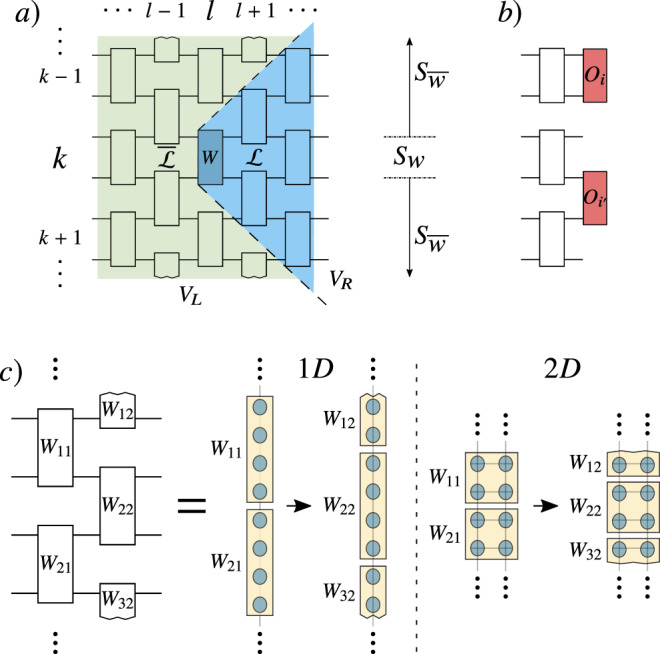
Alternating Layered Ansatz.
a Each block Wkl acts on m qubits and is parametrized via (27). As shown, we define Sk as the m-qubit subsystem on which WkL acts, where L is the last layer of V(θ). Given some block W, it is useful for our proofs (outlined in the Methods) to write , where VR contains all gates in the forward light-cone of W. The forward light-cone is defined as all gates with at least one input qubit causally connected to the output qubits of W. We define as the compliment of , Sw as the m-qubit subsystem on which W acts, and as the n − m qubit subsystem on which W acts trivially. b The operator Oi acts nontrivially only in subsystem , while acts nontrivially on the first m/2 qubits of Sk+1, and on the second m/2 qubits of Sk. c Depiction of the Alternating Layered Ansatz with one- and two-dimensional connectivity. Each circle represents a physical qubit.
The index l = 1, …, L in Wkl(θkl) indicates the layer that contains the block, while k = 1, …, ξ indicates the qubits it acts upon. We assume n is a multiple of m, with n = mξ, and that m does not scale with n. As depicted in Fig. 3a, we define Sk as the m-qubit subsystem on which WkL acts, and we define as the set of all such subsystems. Let us now consider a block Wkl(θkl) in the lth layer of the ansatz. For simplicity we henceforth use W to refer to a given Wkl(θkl). As shown in the Methods section, given a θν ∈ θkl that parametrizes a rotation (with σν a Pauli operator) inside a given block W, one can always express
The contribution to the gradient ∇C from a parameter θν in the block W is given by the partial derivative ∂νC. While the value of ∂νC depends on the specific parameters θ, it is useful to compute , i.e., the average gradient over all possible unitaries V(θ) within the ansatz. Such an average may not be representative near the minimum of C, although it does provide a good estimate of the expected gradient when randomly initializing the angles in V(θ). In the Methods Section we explicitly show how to compute averages of the form 〈…〉V, and in the Supplementary Note 3 we provide a proof for the following Proposition.
The average of the partial derivative of any cost function of the form (6) with respect to a parameter θν in a block W of the ansatz in Fig. 3 is
Here we recall that a t-design is an ensemble of unitaries, such that sampling over their distribution yields the same properties as sampling random unitaries from the unitary group with respect to the Haar measure up to the first t moments38. The Methods section provides a formal definition of a t-design.
Proposition 2 states that the gradient is not biased in any particular direction. To analyze the trainability of C, we consider the second moment of its partial derivatives:
Here we present our main theorems and corollaries, with the proofs sketched in the Methods and detailed in the Supplementary Information. In addition, in the Methods section we provide some intuition behind our main results by analyzing a generalization of the warm-up example where V(θ) is composed of a single layer of the ansatz in Fig. 3. This case bridges the gap between the warm-up example and our main theorems and also showcases the tools used to derive our main result.
The following theorem provides an upper bound on the variance of the partial derivative of a global cost function which can be expressed as the expectation value of an operator of the form
Consider a trainable parameter θν in a block W of the ansatz in Fig. 3. Let Var[∂νC] be the variance of the partial derivative of a global cost function C (with O given by (10)) with respect to θν. If WA, WB of (7), and each block in V(θ) form a local 2-design, then Var[∂νC] is upper bounded by
(i)For N = 1 and when each is a non-trivial projector, then defining , we have
(ii)For arbitrary N and when each satisfies and , then
From Theorem 1 we derive the following corollary.
Consider the function Fn(L, l).
(i)Let N = 1 and let each be a non-trivial projector, as in case (i) of Theorem 1. If and if the number of layers , then
(ii)Let N be arbitrary, and let each satisfy and , as in case (ii) of Theorem 1. If , , and if the number of layers , then
Let us now make several important remarks. First, note that part (i) of Corollary 1 includes as a particular example the cost function CG of (1). Second, part (ii) of this corollary also includes as particular examples operators with , as well as . Finally, we remark that Fn(L, l) becomes trivial when the number of layers L is Ω(poly(n)), however, as we discuss below, we can still find that Var[∂νCG] vanishes exponentially in this case.
Our second main theorem shows that barren plateaus can be avoided for shallow circuits by employing local cost functions. Here we consider m-local cost functions where each acts nontrivially on at most m qubits and (on these qubits) can be expressed as :
Consider a trainable parameter θν in a block W of the ansatz in Fig. 3. Let Var[∂νC] be the variance of the partial derivative of an m-local cost function C (with O given by (16)) with respect to θν. WA, WB of (7), and each block in V(θ) form a local 2-design, then Var[∂νC] is lower bounded by
Let us make a few remarks. First, note that the in the lower bound indicates that training V(θ) is easier when is far from the identity. Second, the presence of in Gn(L, l) implies that we have no guarantee on the trainability of a parameter θν in W if ρ is maximally mixed on the qubits in the backwards light-cone.
From Theorem 2 we derive the following corollary for m-local cost functions, which guarantees the trainability of the ansatz for shallow circuits.
Consider the function Fn(L, l). Let O be an operator of the form (16), as in Theorem 2. If at least one term in the sum in (18) vanishes no faster than Ω(1/poly(n)), and if the number of layers L is , then
Hence, when L is there is a transition region where the lower bound vanishes faster than polynomially, but slower than exponentially.
We finally justify the assumption of each block being a local 2-design from the fact that shallow circuit depths lead to such local 2-designs. Namely, it has been shown that one-dimensional 2-designs have efficient quantum circuit descriptions, requiring gates to be exactly implemented38, or to be approximately implemented39,40. Hence, an L-layered ansatz in which each block forms a 2-design can be exactly implemented with a depth , and approximately implemented with . For the case of two-dimensional connectivity, it has been shown that approximate 2-designs require a circuit depth of to be implemented40. Therefore, in this case the depth of the layered ansatz is . The latter shows that increasing the dimensionality of the circuit reduces the circuit depth needed to make each block a 2-design.
Moreover, it has been shown that the Alternating Layered Ansatz of Fig. 3 will form an approximate one-dimensional 2-design on n qubits if the number of layers is 40. Hence, for deep circuits, our ansatz behaves like a random circuit and we recover the barren plateau result of9 for both local and global cost functions.
As an important example to illustrate the cost-function-dependent barren plateau phenomenon, we consider quantum autoencoders11,41–44. In particular, the pioneering VQA proposed in ref. 11 has received significant literature attention, due to its importance to quantum machine learning and quantum data compression. Let us briefly explain the algorithm in ref. 11.
Consider a bipartite quantum system AB composed of nA and nB qubits, respectively, and let be an ensemble of pure states on AB. The goal of the quantum autoencoder is to train a gate sequence V(θ) to compress this ensemble into the A subsystem, such that one can recover each state with high fidelity from the information in subsystem A. One can think of B as the “trash” since it is discarded after the action of V(θ).
To quantify the degree of data compression, ref. 11 proposed a cost function of the form:
To address this issue, we propose the following local cost function
Here we simulate the autoencoder algorithm to solve a simple problem where nA = 1, and where the input state ensemble is given by


In our heuristics, the gate sequence V(θ) is given by two layers of the ansatz in Fig. 4, so that the number of gates and parameters in V(θ) increases linearly with nB. Note that this ansatz is a simplified version of the ansatz in Fig. 3, as we can only generate unitaries with real coefficients. All parameters in V(θ) were randomly initialized and as detailed in the Methods section, we employ a gradient-free training algorithm that gradually increases the number of shots per cost-function evaluation.
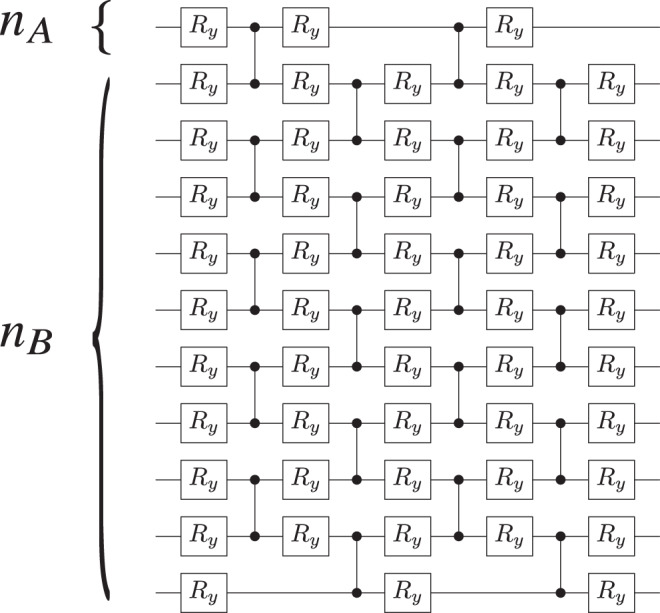
Alternating Layered Ansatz for V(θ) employed in our numerical simulations.
Each layer is composed of control-Z gates acting on alternating pairs of neighboring qubits which are preceded and followed by single qubit rotations around the y-axis, . Shown is the case of two layers, nA = 1, and nB = 10 qubits. The number of variational parameters and gates scales linearly with nB: for the case shown there are 71 gates and 51 parameters. While each block in this ansatz will not form an exact local 2-design, and hence does not fall under our theorems, one can still obtain a cost-function-dependent barren plateau.
Analysis of the n-dependence. Figure 5 shows representative results of our numerical implementations of the quantum autoencoder in ref. 11 obtained by training V(θ) with the global and local cost functions respectively given by (22) and (23). Specifically, while we train with finite sampling, in the figures we show the exact cost-function values versus the number of iterations. Here, the top (bottom) axis corresponds to the number of iterations performed while training with (). For nB = 10 and 15, Fig. 5 shows that we are able to train V(θ) for both cost functions. For nB = 20, the global cost function initially presents a plateau in which the optimizing algorithm is not able to determine a minimizing direction. However, as the number of shots per function evaluation increases, one can eventually minimize . Such result indicates the presence of a barren plateau where the gradient takes small values which can only be detected when the number of shots becomes sufficiently large. In this particular example, one is able to start training at around 140 iterations.

Cost versus number of iterations for the quantum autoencoder problem defined by Eqs. (25)–(26).
In all cases we employed two layers of the ansatz shown in Fig. 4, and we set nA = 1, while increasing nB = 10, 15, …, 100. The top (bottom) axis corresponds to the global cost function of Eq. (22) (local cost function of (23)). As can be seen, can be trained up to nB = 20 qubits, while trained in all cases. These results indicate that global cost function presents a barren plateau even for a shallow depth ansatz, and this can be avoided by employing a local cost function.
When nB > 20 we are unable to train the global cost function, while always being able to train our proposed local cost function. Note that the number of iterations is different for and , as for the global cost function case we reach the maximum number of shots in fewer iterations. These results indicate that the global cost function of (22) exhibits a barren plateau where the gradient of the cost function vanishes exponentially with the number of qubits, and which arises even for constant depth ansatzes. We remark that in principle one can always find a minimizing direction when training , although this would require a number of shots that increases exponentially with nB. Moreover, one can see in Fig. 5 that randomly initializing the parameters always leads to due to the narrow gorge phenomenon (see Proposition 1), i.e., where the probability of being near the global minimum vanishes exponentially with nB.
On the other hand, Fig. 5 shows that the barren plateau is avoided when employing a local cost function since we can train for all considered values of nB. Moreover, as seen in Fig. 5, can be trained with a small number of shots per cost-function evaluation (as small as 10 shots per evaluation).
Analysis of the L-dependence. The power of Theorem 2 is that it gives the scaling in terms of L. While one can substitute a function of n for L as we did in Corollary 2, one can also directly study the scaling with L (for fixed n). Figure 6 shows the dependence on L when training for the autoencoder example with nA = 1 and nB = 10. As one can see, the training becomes more difficult as L increases. Specifically, as shown in the inset it appears to become exponentially more difficult, as the number of shots needed to achieve a fixed cost value grows exponentially with L. This is consistent with (and hence verifies) our bound on the variance in Theorem 2, which vanishes exponentially in L, although we remark that this behavior can saturate for very large L9.
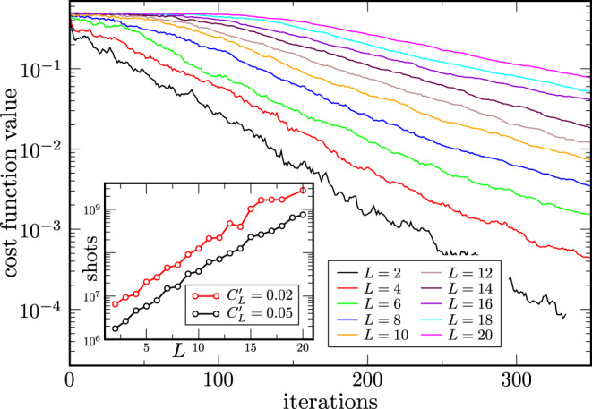
Local cost versus number of iterations for the quantum autoencoder problem in Eqs. (25–26) with nB = 10.
Each curve corresponds to a different number of layers L in the ansatz of Fig. 4 with L = 2,…, 20. Curves were averaged over 9 instances of the autoencoder. As the number of layers increases, the optimization becomes harder. Inset: Number of shots needed to reach cost values of and versus number of layers L. As L increases the number of shots needed to reach the indicated cost values appears to increase exponentially.
In summary, even though the ansatz employed in our heuristics is beyond the scope of our theorems, we still find cost-function-dependent barren plateaus, indicating that the cost-function dependent barren plateau phenomenon might be more general and go beyond our analytical results.
While scaling results have been obtained for classical neural networks45, very few such results exist for the trainability of parametrized quantum circuits, and more generally for quantum neural networks. Hence, rigorous scaling results are urgently needed for VQAs, which many researchers believe will provide the path to quantum advantage with near-term quantum computers. One of the few such results is the barren plateau theorem of ref. 9, which holds for VQAs with deep, hardware-efficient ansatzes.
In this work, we proved that the barren plateau phenomenon extends to VQAs with randomly initialized shallow Alternating Layered Ansatzes. The key to extending this phenomenon to shallow circuits was to consider the locality of the operator O that defines the cost function C. Theorem 1 presented a universal upper bound on the variance of the gradient for global cost functions, i.e., when O is a global operator. Corollary 1 stated the asymptotic scaling of this upper bound for shallow ansatzes as being exponentially decaying in n, indicating a barren plateau. Conversely, Theorem 2 presented a universal lower bound on the variance of the gradient for local cost functions, i.e., when O is a sum of local operators. Corollary 2 notes that for shallow ansatzes this lower bound decays polynomially in n. Taken together, these two results show that barren plateaus are cost-function-dependent, and they establish a connection between locality and trainability.
In the context of chemistry or materials science, our present work can inform researchers about which transformation to use when mapping a fermionic Hamiltonian to a spin Hamiltonian46, i.e., Jordan-Wigner versus Bravyi–Kitaev47. Namely, the Bravyi–Kitaev transformation often leads to more local Pauli terms, and hence (from Corollary 2) to a more trainable cost function. This fact was recently numerically confirmed48.
Moreover, the fact that Corollary 2 is valid for arbitrary input quantum states may be useful when constructing variational ansatzes. For example, one could propose a growing ansatz method where one appends layers of the hardware-efficient ansatz to a previously trained (hence fixed) circuit. This could then lead to a layer-by-layer training strategy where the previously trained circuit can correspond to multiple layers of the same hardware-efficient ansatz.
We remark that our definition of a global operator (local operator) is one that is both non-local (local) and many body (few body). Therefore, the barren plateau phenomenon could be due to the many-bodiness of the operator rather than the non-locality of the operator; we leave the resolution of this question to future work. On the other hand, our Theorem 1 rules out the possibility that barren plateaus could be due to cardinality, i.e., the number of terms in O when decomposed as a sum of Pauli products49. Namely, case (ii) of this theorem implies barren plateaus for O of essentially arbitrary cardinality, and hence cardinality is not the key variable at work here.
We illustrated these ideas for two examples VQAs. In Fig. 2, we considered a simple state-preparation example, which allowed us to delve deeper into the cost landscape and uncover another phenomenon that we called a narrow gorge, stated precisely in Proposition 1. In Fig. 5, we studied the more important example of quantum autoencoders, which have generated significant interest in the quantum machine learning community. Our numerics showed the effects of barren plateaus: for more than 20 qubits we were unable to minimize the global cost function introduced in11. To address this, we introduced a local cost function for quantum autoencoders, which we were able to minimize for system sizes of up to 100 qubits.
There are several directions in which our results could be generalized in future work. Naturally, we hope to extend the narrow gorge phenomenon in Proposition 1 to more general VQAs. In addition, we hope in the future to unify our theorems 1 and 2 into a single result that bounds the variance as a function of a parameter that quantifies the locality of O. This would further solidify the connection between locality and trainability. Moreover, our numerics suggest that our theorems (which are stated for exact 2-designs) might be extendable in some form to ansatzes composed of simpler blocks, like approximate 2-designs39.
We emphasize that while our theorems are stated for a hardware-efficient ansatz and for costs that are of the form (6), it remains an interesting open question as to whether other ansatzes, cost function, and architectures exhibit similar scaling behavior as that stated in our theorems. For instance, we have recently shown50 that our results can be extended to a more general type of Quantum Neural Network called dissipative quantum neural networks51. Another potential example of interest could be the unitary-coupled cluster (UCC) ansatz in chemistry52, which is intended for use in the depth regime34. Therefore it is important to study the key mathematical features of an ansatz that might allow one to go from trainability for depth (which we guarantee here for local cost functions) to trainability for depth.
Finally, we remark that some strategies have been developed to mitigate the effects of barren plateaus32,33,53,54. While these methods are promising and have been shown to work in certain cases, they are still heuristic methods with no provable guarantees that they can work in generic scenarios. Hence, we believe that more work needs to be done to better understand how to prevent, avoid, or mitigate the effects of barren plateaus.
In this section, we provide additional details for the results in the main text, as well as a sketch of the proofs for our main theorems. We note that the proof of Theorem 2 comes before that of Theorem 1 since the latter builds on the former. More detailed proofs of our theorems are given in the Supplementary Information.
Let us first discuss the formulas we employed to compute Var[∂νC]. Let us first note that without loss of generality, any block Wkl(θkl) in the Alternating Layered Ansatz can be written as a product of ζkl independent gates from a gate alphabet as
For the proofs of our results, it is helpful to conceptually break up the ansatz as follows. Consider a block Wkl(θkl) in the lth layer of the ansatz. For simplicity, we henceforth use W to refer to a given Wkl(θkl). Let Sw denote the m-qubit subsystem that contains the qubits W acts on, and let be the (n − m) subsystem on which W acts trivially. Similarly, let and denote the Hilbert spaces associated with Sw and , respectively. Then, as shown in Fig. 3a, V(θ) can be expressed as
Let us here recall that the Alternating Layered Ansatz can be implemented with either a 1D or 2D square connectivity as schematically depicted in Fig. 3c. We remark that the following results are valid for both cases as the light-cone structure will be the same. Moreover, the notation employed in our proofs applies to both the 1D and 2D cases. Hence, there is no need to refer to the connectivity dimension in what follows.
Let us now assume that θν is a parameter inside a given block W, we obtain from (6), (27), and (28)

Finally, from (29) we can derive a general formula for the variance:
Here we introduce the main tools employed to compute quantities of the form 〈…〉V. These tools are used throughout the proofs of our main results.
Let us first remark that if the blocks in V(θ) are independent, then any average over V can be computed by averaging over the individual blocks, i.e., . For simplicity let us first consider the expectation value over a single block W in the ansatz. In principle 〈…〉W can be approximated by varying the parameters in W and sampling over the resulting 2m × 2m unitaries. However, if W forms a t-design, this procedure can be simplified as it is known that sampling over its distribution yields the same properties as sampling random unitaries from the unitary group with respect to the unique normalized Haar measure.
Explicitly, the Haar measure is a uniquely defined left and right-invariant measure over the unitary group dμ(W), such that for any unitary matrix A ∈ U(2m) and for any function f(W) we have

From the general form of C in Eq. (6) we can see the cost function is a polynomial of degree at most 2 in the matrix elements of each block Wkl in V(θ), and at most 2 in those of . Then, if a given block W forms a 2-design, one can employ the following elementwise formula of the Weingarten calculus55,56 to explicitly evaluate averages over W up to the second moment:

The goal of this section is to provide some intuition for our main results. Specifically, we show here how the scaling of the cost function variance can be related to the number of blocks we have to integrate to compute , the locality of the cost functions, and with the number of layers in the ansatz.
First, we recall from Eq. (38) that integrating over a block leads to a coefficient of the order 1/22m. Hence, we see that the more blocks one integrates over, the worse the scaling can be.
We now generalize the warm-up example. Let V(θ) be a single layer of the alternating ansatz of Fig. 3, i.e., V(θ) is a tensor product of m-qubit blocks Wk: = Wk1, with k = 1, …, ξ (and with ξ = n/m), so that θν is in the block . In the Supplementary Note 5 we generalize this scenario to the when the input state is not , but instead is an arbitrary state ρ.
From (31), the partial derivative of the global cost function in (1) can be expressed as
On the other hand, for a local cost let us consider a single term in (3) where , so that
Let us now briefly provide some intuition as to why the scaling of local cost gradients becomes exponentially vanishing with the number of layers as in Theorem 2. Consider the case when V(θ) contains L layers of the ansatz in Fig. 3. Moreover, as shown in Fig. 7, let W be in the first layer, and let Oi act on the m topmost qubits of . As schematically depicted in Fig. 7, we now have to integrating over L − 1 blocks. Then, as proved in the Supplementary Note 5, integrating over a block leads to a coefficient 2m/2/(2m + 1). Hence, after integrating L − 1 times, we obtain a coefficient which vanishes no faster than if .
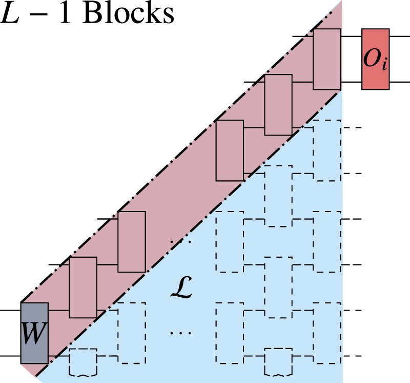
The block W is in the first layer of V(θ), and the operator Oi acts on the topmost m qubits in the forward light-cone of W.
Dashed thick lines indicate the backward light-cone of Oi. All but L − 1 blocks simplify to identity in Ωqp of Eq. (34).
As we discuss below, for more general scenarios the computation of Var[∂νC] becomes more complex.
Here we present a sketch of the proof of Theorems 1 and 2. We refer the reader to the Supplementary Information for a detailed version of the proofs.
As mentioned in the previous subsection, if each block in V(θ) forms a local 2-design, then we can explicitly calculate expectation values 〈…〉W via (38). Hence, to compute , and in (31), one needs to algorithmically integrate over each block using the Weingarten calculus. In order to make such computation tractable, we employ the tensor network representation of quantum circuits.
For the sake of clarity, we recall that any two-qubit gate can be expressed as , where Uijkl is a 2 × 2 × 2 × 2 tensor. Similarly, any block in the ansatz can be considered as a tensor. As schematically shown in Fig. 8a, one can use the circuit description of and Ψpq to derive the tensor network representation of terms such as . Here, is obtained from (34) by simply replacing O with Oi.
![Tensor-network representations of the terms relevant to Var[∂νC].](/dataresources/secured/content-1766026812779-4b117794-906d-409b-a169-b645eb519aa0/assets/41467_2021_21728_Fig8_HTML.jpg)
Tensor-network representations of the terms relevant to Var[∂νC].
a Representation of of Eq. (34) (left), where the superscript indicates that O is replaced by Oi. In this illustration, we show the case of n = 2m qubits, and we denote . We also show the representation of (middle) and of (right). b By means of the Weingarten calculus we can algorithmically integrate over each block in the ansatz. After each integration one obtains four new tensors according to Eq. (38). Here we show the tensor obtained after the integrations and , which are needed to compute as in Eq. (31). c As shown in the Supplementary Note 1, the result of the integration is a sum of the form (49), where the deltas over p, q, , and arise from the contractions between Ppq and .
In Fig. 8b we depict an example where we employ the tensor network representation of to compute the average of , and . As expected, after each integration one obtains a sum of four new tensor networks according to Eq. (38).
Let us first consider an m-local cost function C where O is given by (16), and where acts nontrivially in a given subsystem Sk of . In particular, when is of this form the proof is simplified, although the more general proof is presented in the Supplementary Note 6. If we find , and hence
Then, as shown in the Supplementary Information
By employing properties of DHS one can show (see Supplementary Note 6)
Let us now provide a sketch of the proof of Theorem 1, case (i). Here we denote for simplicity . We leave the proof of case (ii) for the Supplementary Note 7. In this case there are now operators Oi which act outside of the forward light-cone of W. Hence, it is convenient to include in VR not only all the gates in but also all the blocks in the final layer of V(θ) (i.e., all blocks WkL, with k = 1, …ξ). We can define as the compliment of , i.e., as the subsystem of all qubits which are not in (with associated Hilbert-space ). Then, we have and , where we define , , and . Here, we define and , which are the set of indices whose associated qubits are inside and outside , respectively. We also write , where we define and .
Using the fact that the blocks in V(θ) are independent we can now compute . Then, from the definition of Ωpq in Eq. (34) and the fact that one can always express

On the other hand, as shown in the Supplementary Note 7 (and as schematically depicted in Fig. 8c), when computing the expectation value in (47), one obtains
Here we describe the gradient-free optimization method used in our heuristics. First, we note that all the parameters in the ansatz are randomly initialized. Then, at each iteration, one solves the following sub-space search problem: , where A is a randomly generated isometry, and s = (s1, …, sd) is a vector of coefficients to be optimized over. We used d = 10 in our simulations. Moreover, the training algorithm gradually increases the number of shots per cost-function evaluation. Initially, C is evaluated with 10 shots, and once the optimization reaches a plateau, the number of shots is increased by a factor of 3/2. This process is repeated until a termination condition on the value of C is achieved, or until we reach the maximum value of 105 shots per function evaluation. While this is a simple variable-shot approach, we remark that a more advanced variable-shot optimizer can be found in ref. 57.
Finally, let us remark that while we employ a sub-space search algorithm, in the presence of barren plateaus all optimization methods will (on average) fail unless the algorithm has a precision (i.e., number of shots) that grows exponentially with n. The latter is due to the fact that an exponentially vanishing gradient implies that on average the cost function landscape will essentially be flat, with the slope of the order of . Hence, unless one has a precision that can detect such small changes in the cost value, one will not be able to determine a cost minimization direction with gradient-based, or even with black-box optimizers such as the Nelder–Mead method58–61.
The online version contains supplementary material available at 10.1038/s41467-021-21728-w.
We thank Jacob Biamonte, Elizabeth Crosson, Burak Sahinoglu, Rolando Somma, Guillaume Verdon, and Kunal Sharma for helpful conversations. All authors were supported by the Laboratory Directed Research and Development (LDRD) program of Los Alamos National Laboratory (LANL) under project numbers 20180628ECR (for M.C.), 20190065DR (for A.S., L.C., and P.J.C.), and 20200677PRD1 (for T.V.). M.C. and A.S. were also supported by the Center for Nonlinear Studies at LANL. P.J.C. acknowledges initial support from the LANL ASC Beyond Moore’s Law project. This work was also supported by the U.S. Department of Energy (DOE), Office of Science, Office of Advanced Scientific Computing Research, under the Quantum Computing Application Teams program.
The project was conceived by M.C., L.C., and P.J.C. The manuscript was written by M.C., A.S., T.V., L.C., and P.J.C. T.V. proved Proposition 1. M.C. and A.S. proved Proposition 2 and Theorems 1–2. M.C., A.S., T.V., and P.J.C. proved Corollaries 1–2. M.C., A.S., T.V., L.C., and P.J.C. analyzed the quantum autoencoder. For the numerical results, T.V. performed the simulation in Fig. 2, and L.C. performed the simulation in Fig. 5.
Data generated and analyzed during the current study are available from the corresponding author upon reasonable request.
The authors declare no competing interests.
1.
2.
3.
4.
5.
6.
7.
8.
9.
10.
11.
12.
13.
14.
15.
16.
17.
18.
19.
20.
21.
22.
23.
24.
25.
26.
27.
28.
29.
30.
31.
32.
33.
34.
35.
36.
37.
38.
39.
40.
41.
42.
43.
44.
45.
46.
47.
48.
49.
50.
51.
52.
53.
54.
55.
56.
57.
58.
59.
60.
61.
 Cost function dependent barren plateaus in shallow parametrized quantum circuits
 Facebook
 Twitter
 Linkedin
 Whatsapp

