Method overview

BayesS is a method that can estimate three key parameters to describe the genetic architecture of complex traits by a Bayesian mixed linear model¹³, namely SNP-based heritability ($$ h_{\mathrm{SNP}}^2$$), polygenicity (π) and the relationship between MAF and effect size (S), all of which are defined with respect to a certain set of SNPs (see the definition of $$ h_{\mathrm{SNP}}^2$$ as an example⁵). BayesS requires individual-level data. SBayesS is an extension of BayesS, but only requires GWAS summary statistics of the SNPs and LD information from a reference sample (see the “Methods” section, Supplementary Note and Supplementary Fig. 1). We compute pairwise LD correlations between SNPs located on the same chromosome from a reference sample and remove correlations that can be attributed to sampling variation by a chi-squared test, resulting in a sparse LD matrix (see the “Methods” section). In addition, we model analytically the sampling variance of LD estimates as part of the residual variance and allow the estimate of residual variance to vary across SNPs (Supplementary Note). Compared to BayesS, SBayesS not only addresses the barrier of data sharing as it does not require individual-level data, but also substantially increases the computational efficiency because of the use of sparse LD matrix and a different updating strategy in the MCMC sampling (Supplementary Note). These features allow SBayesS to be scalable to data with millions of SNPs regardless of the discovery GWAS sample sizes. To examine the convergence of MCMC, we provide a GCTB-SBayesS implementation of the Gelman–Rubin statistic²⁷ which compares the variation between and within multiple chains with different starting values of the model parameters (see the “Methods” section). Convergence is only concluded if all the three key parameters converge, which may not occur if the LD matrix from a reference sample is too divergent from that of the GWAS sample, or if the summary statistics are generated from a GWAS with low power or contain uncorrected population stratification, poor imputation or other errors such as misreported per-SNP sample size and allele frequency.

In light of recent studies^11,28, which point out a possible lack of fit of a point–normal mixture model to some traits, we further extended SBayesS to a multi-component mixture model (referred to as SBayesRS), following the framework of SBayesR²⁹. In SBayesRS, each SNP effect is assumed to have a mixture of a point mass at zero and three normal distributions with mean zero and variances that differ by a factor of 10 (see the “Methods” section). This flexible prior accounts for a more complex genetic architecture with a spectrum of very small to very large effect sizes. The S parameter and overall polygenicity are estimated based on the SNPs across all nonnull mixture components.

To better understand the variability of regional genetic architecture in different parts of the genome, we incorporate functional genomic annotations into SBayesS to allow the three key parameters to vary in different annotation categories, e.g., coding, regulatory and repressed regions. We performed the functional partitioning SBayesS analysis (denoted SBayesS-strat) based on a two-component model that fitted SNPs in one annotation as the first component and the rest of the SNPs as the second component (see the “Methods” section). During MCMC sampling, the enrichment of a parameter in an annotation category is computed as the ratio of the sampled value of the parameter in the category to that for the whole genome (see the “Methods” section).

Benchmarking SBayesS with BayesS

We ran both SBayesS and BayesS with ~1.1 million HapMap3 SNPs with MAF ≥ 0.01 for 18 quantitative traits (n > 100k) as analysed in Zeng et al. ¹³. We used the HapMap3 SNPs as they were optimised to tag common genetic variants³⁰ and are widely used in the literature which improves the comparability of our results with those generated using published GWAS summary statistics. Hence, the reported parameters are specific to this SNP set. For ease of computation, we used unrelated individuals of European ancestry from the interim release of the UKB data for the BayesS analysis (maximum n = 120k across traits) and the same data to generate GWAS summary statistics for the SBayesS analysis. We show in Fig. 1 that the correlation between the SBayesS and BayesS estimates for all of the three genetic architecture parameters was close to one across traits (Pearson correlation r = 0.998 for $$ h_{\mathrm{SNP}}^2$$, 0.985 for π and 0.965 for S).

Fig. 1

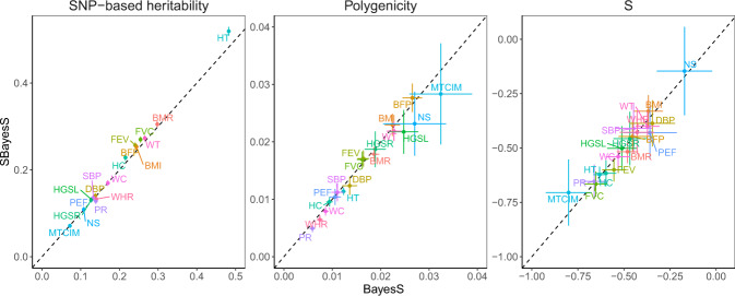
Benchmarking SBayesS with BayesS using the same data for 18 UKB traits.

Three genetic architecture parameters were compared, i.e., SNP-based heritability, polygenicity (defined as proportion of SNPs with nonzero effects) and S (defined as relationship between MAF and effect size), based on the unrelated individuals of European ancestry in the interim release of the UKB data (max n = 120k) and ~1.1 million HapMap3 common SNPs (MAF > 0.01). The sparse LD matrix used in SBayesS was computed from a random sample of 50k unrelated individuals from the full UKB cohort at a chi-squared threshold of 10 (corresponding to a LD r² threshold of 2 × 10⁻⁴). Data are presented as posterior means ± posterior standard errors. The traits are indicated by different colours labelled with their acronyms. BMR basal metabolic rate, BMI body mass index, BFP body fat percentage, DBP diastolic blood pressure, FEV forced expiratory volume, FVC forced vital capacity, HGSL hand grip strength (left), HGSR hand grip strength (right), HCadjBMI hip circumference adjusted for BMI, HT height, MTCIM mean time to correctly identify matches, NS neuroticism score, PEF peak expiratory flow, PR pulse rate, SBP systolic blood pressure, WCadjBMI waist circumference adjusted for BMI, WHRadjBMI waist–hip ratio adjusted for BMI, WT weight.

We performed additional sensitivity analyses to investigate the impact of the sparsity of LD matrix, the SNP panel, the choice of reference sample and the reference sample size on the performance of SBayesS. We found that SBayesS was robust to different chi-squared thresholds used for LD filtering (Supplementary Fig. 2) and gave consistent results with BayesS regardless of whether using HapMap3 (Fig. 1) or UKB Axiom array panel (Supplementary Fig. 3a). The analysis using HapMap3 SNPs tended to give slightly lower $$ {\widehat{h}}_{\mathrm{SNP}}^2$$ and $$ \widehat{\pi }$$ but stronger signals of S for both SBayesS and BayesS (Supplementary Fig. 3b, c), possibly due to the under-representation of low-frequency SNPs in HapMap3 panel in comparison with the UKB Axiom array panel (Supplementary Fig. 4). There was negligible difference in parameter estimates when the LD reference sample size (n_ref) decreased from 50k to 20k but notable inflation in $$ {\widehat{h}}_{\mathrm{SNP}}^2$$ and $$ \widehat{S}$$ when n_ref further decreased to 4k (Supplementary Fig. 5), suggesting that the LD reference sample size cannot be too small relative to the GWAS sample size. Given a constant reference sample size (n_ref = 50k), we ran GWAS with sample sizes n_gwas = 120k and 350k and found highly consistent parameter estimates between SBayesS and BayesS regardless of n_gwas (Supplementary Fig. 6). As expected, the π estimate from either SBayesS or BayesS increased with larger n_gwas because of the increased power to detect small effects, consistent with the observation from an independent prior study²⁸. Since $$ h_{\mathrm{SNP}}^2$$ and S were estimated based on the SNPs with nonzero effects, the estimators of these parameters were also to some extent sample size dependent (see Supplementary Note for more discussion). Furthermore, with both n_ref = 50k and n_gwas = 300k held constant, we benchmarked BayesS and SBayesS in a few different scenarios where the LD reference was a subset of the GWAS sample, an independent sample from the same or slightly different population, or a sample of different ancestry. The performance of SBayesS was almost independent of the overlap between the GWAS and LD reference samples as long as they are from the same population but started to deteriorate when the genetic discrepancy between GWAS and reference samples increased (Supplementary Fig. 8). This observation demonstrates the importance of choosing a reference sample that is genetically as close to the GWAS sample as possible in the analysis of summary data³¹.

The parameter estimates were largely consistent between SBayesS and SBayesRS except for polygenicity, of which the estimate from SBayesRS was higher than that from SBayesS (Supplementary Fig. 9a). This is because, on one hand, SBayesS has a relatively low power to detect SNPs with very small effect sizes due to its assumption of a single normal distribution; on the other hand, SBayesRS tends to overestimate the number of SNPs with very small effect sizes due to the insufficient power to distinguish very small effect sizes from zero, as suggested by simulation (Supplementary Fig. 9c). Nevertheless, the number of SNPs with relatively large effects estimated from SBayesS was mostly consistent with that from SBayesRS (Supplementary Fig. 9b).

Finally, we tested the method in application to ascertained case-control data by simulation. The parameter estimates were nearly unbiased regardless of whether cases were oversampled, although the sampling variances of the estimates of polygenicity and S were relatively large in some simulation scenarios where the number of cases was relatively small (Supplementary Fig. 10).

Analyses of GWAS summary data from the UKB and other published studies

We applied SBayesS to analyse the full release of the UKB data, including 26 complex traits and 9 common diseases (Supplementary Table 1). Although individual-level data are available in the UKB, application of the standard BayesS to ~350k unrelated individuals with ~1.1 million HapMap3 SNPs is computationally prohibitive. Prior to running SBayesS, we carried out standard quality control (QC) of the data (see the “Methods” section) and used linear regression to perform a GWAS analysis in unrelated individuals to generate summary statistics for each trait. We also applied SBayesS to data for 9 other complex common diseases from published GWAS of very large sample size where only summary statistics are available (Supplementary Table 2). In the analysis of the UKB data, we used the sparse LD matrix computed from a random sample of 50k unrelated individuals. For the analysis of data from published GWAS of which nearly all the samples are of European ancestry, the GERA³² sample was used as the LD reference. To mitigate the problem due to inconsistent LD between the GWAS and reference samples, we excluded SNPs in the major histocompatibility complex (MHC) region although the SBayesS results with and without the MHC region were very similar (Supplementary Fig. 11). The SNP-based heritability estimates for the diseases were converted to those on the liability scale³³.

On average across the 44 complex traits (including diseases), 1.8% of the 1.1 million common HapMap3 SNPs explained 18% of the phenotypic variance (Fig. 2 and Supplementary Tables 1, 2). The estimate of $$ h_{\mathrm{SNP}}^2$$ for height was 0.545 (posterior standard error or p.s.e. = 0.003), consistent with those in previous studies using different approaches and data sets^6,14,34–36. The most polygenic traits (i.e., body fat percentage, educational attainment and schizophrenia) had about 5% (~55,000) SNPs with nonzero effects. The least polygenic traits were prostate cancer, age at menopause and male pattern baldness, which were affected by about 0.1–0.3% (1000–3000) common SNPs. The estimate of S was significantly negative (P < 0.001) in all the traits analysed (median $$ \widehat{S}$$ = −0.578, SD = 0.096), suggesting a pervasive action of negative selection on the trait-associated variants. We also re-ran the analysis for the 9 public GWAS data sets with the UKB subsample as the LD reference and found that the results were highly consistent with those using LD from the GERA (Supplementary Fig. 12).

Fig. 2

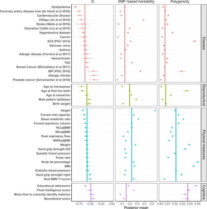
Estimation of the three genetic architecture parameters for 35 traits from the UKB and 9 common diseases from published GWAS.

Shown are the posterior means (dots) and standard errors (horizontal bars) of the parameters for each trait. The colour indicates the UKB trait category that the trait belongs to. The vertical bar shows the median of the estimates across traits in each category.

We used the UKB classification code to classify the 44 traits into four categories related to disease, reproduction, physical measures, and cognition (Supplementary Table 3). The estimates of the genetic architecture parameters varied across traits and appeared to have distinct patterns in different categories (Fig. 2). Physical measures had the highest median SNP-based heritability (0.225), followed by reproductive traits (0.197). The median polygenicity estimate was the lowest for diseases (0.007) and reproductive traits (0.008) and the highest for cognitive traits (0.037). The estimates of polygenicity for psychiatric disorders such as schizophrenia ($$ \widehat{\pi }$$= 0.046, p.s.e. = 0.003) and bipolar disorder ($$ \widehat{\pi }$$ = 0.034, p.s.e. = 0.009) were substantially higher than that for other types of disease and comparable to those for the cognitive traits, consistent with the high polygenicity for brain-related traits reported in previous studies^11,28. The absolute median value of $$ \widehat{S}$$ was the highest for diseases, especially cardiovascular diseases, and the lowest for cognitive traits, with a relatively large variability in $$ \widehat{S}$$ for diseases. We observed similar results from SBayesRS but with higher $$ \widehat{\pi }$$ (Supplementary Fig. 13), in line with the observations from the benchmark analysis above.

To investigate the diversity of genetic architecture in more traits, we applied SBayesS to GWAS summary data from the Neale Lab (http://www.nealelab.is/uk-biobank) for 274 UKB traits, among which 130 passed the convergence test and 110 of these were not included in the analyses above (Supplementary Table 4). The traits that failed to converge tended to have much smaller sample size or $$ {\widehat{h}}_{\mathrm{SNP}}^2$$ compared to the ones that converged (mean n = 231k and $$ {\widehat{h}}_{\mathrm{SNP}}^2=0.223$$ for the converged vs. mean n = 73k and $$ {\widehat{h}}_{\mathrm{SNP}}^2=0.044$$ for the non-converged), but we did not filter traits by $$ {\widehat{h}}_{\mathrm{SNP}}^2$$ to avoid direct ascertainment bias. Figure 3 shows the distributions of the estimated genetic architecture parameters for the total 155 traits (including 18 common diseases) from the UKB and published GWAS. Similar to that for the 44 traits analysed above, the distribution of $$ \widehat{S}$$ appeared symmetric at about −0.6, with 79% of the estimates within the range of −0.7 to −0.5 (median = −0.576) across traits.

Fig. 3

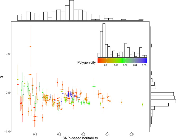
Estimation of the genetic architecture parameters for 155 complex traits.

Shown are the results from the SBayesS analyses using summary data for 130 traits from the Neale Lab and 25 traits from our GWAS analyses and other published studies. The estimated S is plotted against the estimated SNP-based heritability with the histograms showing the marginal distributions of the estimates. Data are presented as posterior means ± posterior standard errors. Colour indicates the estimate of polygenicity for each trait where the scale and distribution are shown in the inset graph.

Prediction of evolutionary parameters for complex traits

Although a negative estimate of S is a signature of negative selection, the numeric interpretation of $$ \widehat{S}$$ is still not clear. For example, our results showed that most traits had $$ \widehat{S}$$ at about −0.6; does it mean that negative selection acted on the associated variants with similar selection strength among traits? To answer this question, we performed forward simulations²⁶ to study the variational patterns of the genetic architecture parameters in a variety of evolutionary scenarios. We focused on three main evolutionary parameters: average selection coefficient ($$ \overline{s}$$), proportion of mutational targets (π_m, i.e., the proportion of DNA sequence at which mutations can affect the trait) and mutational heritability ($$ h_{\mathrm{m}}^2={\sigma }_{\mathrm{m}}^2/{\sigma }_{\mathrm{e}}^2$$ with $$ {\sigma }_{\mathrm{m}}^2$$ being the amount of additional additive genetic variance arising from new mutations in each generation and $$ {\sigma }_{\mathrm{e}}^2$$ being the environmental variance $$ {\sigma }_{\mathrm{e}}^2$$), and set a large range of values for each parameter (see the “Methods” section). The simulations were carried out based on a 100-Mb genome with a variable effective population size inferred from a demographic model³⁷. The selection coefficients were sampled from either a normal distribution or a mixture distribution of many small and some very large values. In the last generation of selection, we used two pleiotropic models (the Simon et al.¹² and Eyre-Walker³ model) to generate causal effects of the mutations on the focal trait (see the “Methods” section). Based on the LD correlation matrix computed from the unrelated individuals in the final generation of the simulated data, we directly simulated GWAS summary statistics with an equal sample size as in the UKB data analysis^11,38 (see the “Methods” section). The genetic architecture parameters $$ h_{\mathrm{SNP}}^2$$, π and S were estimated by SBayesS and SBayesRS using 36k SNPs randomly sampled from the common sequence variants, a comparable SNP density to that of the 1.1 million HapMap3 common SNPs used in the real trait analysis (1.1 × 10⁶ × 1 × 10⁸/3 × 10⁹ = 36,000).

Repeating the simulation with different values of $$ \overline{s}$$, π_m and $$ h_{\mathrm{m}}^2$$ produced a landscape of the genetic architecture under different scenarios (Fig. 4). Our results showed that $$ ∣\widehat{S}∣$$, $$ \widehat{\pi }$$ and $$ {\widehat{h}}_{\mathrm{SNP}}^2$$ increased with the increasing levels of the corresponding evolutionary parameters $$ \overline{s}$$, π_m and $$ h_{\mathrm{m}}^2$$, respectively. The results were generally consistent regardless of the use of SNPs (36k common SNPs or the actual common causal variants), estimation method (SBayesS or SBayesRS), simulation model (the Simons et al. or Eyre-Walker model), or the underlying distribution of selection coefficients (mixture or normal distribution) (Fig. 4 and Supplementary Figs. 14–17). In addition to the direct impact of the evolutionary parameters on the corresponding genetic architecture parameters, $$ \overline{s}$$ had negative effects on $$ {\widehat{h}}_{\mathrm{SNP}}^2$$ and $$ \widehat{\pi }$$ because of causal variants with large effect sizes were purged by negative selection. Using a linear regression analysis of the true causal effects, we obtained the ordinary least-squares (OLS) estimate of S and used it as a proxy of the true value (see the “Methods” section). Regarding to the different distributions of selection coefficients, the true values of S were not highly correlated (Supplementary Fig. 18; r = 0.628), suggesting the distribution of selection coefficient plays a role in determining S. Compared to the true value of S, the SBayesS estimate based on the causal variant genotypes tended to be more negative when selection strength was weak and selection coefficients followed a mixture distribution (Fig. 4). This is because SBayesS assumes normality of the SNP effects whereas the true distribution is a multi-component mixture, supported by our results of maximum-likelihood estimation assuming normality (Supplementary Note and Supplementary Fig. 19). Compared to SBayesS, SBayesRS is more robust to the distribution of causal effects in the estimation of the S parameter (Fig. 4 and Supplementary Fig. 17).

Fig. 4

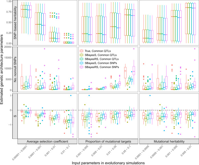
Variational patterns of the estimated genetic architecture parameters under different scenarios of evolutionary simulations.

The selection coefficients followed a mixture distribution, and the Simons et al. pleiotropic model with n_t = 1 was used to generate genetic effects (see the “Methods” section). The x-axis shows the values of three input parameters in the evolutionary simulations. The y-axis shows the distribution of the genetic architecture parameter estimates, where the polygenicity parameter is represented by the number of nonnull SNPs for better benchmarking. Colours indicate the following methods: “True, Common QTLs”—parameters computed directly from the simulated genetic effects of all common causal variants; “SBayesS, Common QTLs” (or “SBayesRS, Common QTLs”)—SBayesS (or SBayesRS) estimates using the genotype data of the common causal variants, “SBayesS, Common SNPs” (or “SBayesRS, Common SNPs”)—SBayesS (or SBayesRS) estimates using the genotype data of 36k common SNPs. Each box plot shows the results of 25 independent simulation replicates. The band inside the box is the median, the bottom and top of the box are the first and third quartiles, respectively (Q1 and Q3), and the lower and upper whiskers are Q1–1.5 × IQR and Q3 + 1.5 × IQR, respectively, where IQR = Q3–Q1.

Next, we used a polynomial regression model to associate the evolutionary parameters ($$ \overline{s}$$, π_m and $$ h_{\mathrm{m}}^2$$) with $$ {\widehat{h}}_{\mathrm{SNP}}^2$$, $$ \widehat{\pi }$$ and $$ \widehat{S}$$ in the entire simulation dataset, and leveraged this association to predict the evolutionary parameters in real data (see the “Methods” section). We demonstrated by a cross-validation analysis in the simulated data that the three evolutionary parameters can be predicted with reasonably high accuracy (Supplementary Fig. 20). We then applied this prediction model to the 44 traits analysed above. Overall, the real trait prediction results were robust to the evolutionary model used for training data simulation and the statistical method for genetic architecture parameter estimation (Fig. 5). Here, we focus on the results from the mixture model for selection coefficients, as similar results were observed from the model assuming normality (Supplementary Fig. 21). The predicted $$ \overline{s}$$ were mostly between 10⁻⁴ and 10⁻³ with a mean of 0.0007 across traits (Fig. 5), in line with the estimates from prior work¹². Cancer, stroke, and coronary artery disease showed the highest predicted $$ \overline{s}$$ (Supplementary Fig. 22), albeit the per-trait $$ \overline{s}$$ had a wide confidence interval which covered a range of possible values by a factor of 10. The predicted π_m was ~1% on average across traits, meaning that ~30 million base pairs of the human genome were mutational targets for a complex trait. The mean predicted $$ h_{\mathrm{m}}^2$$ was 0.001 with relatively small variability across traits comparing to the other two parameters, which can be regarded as a justification of our projection approach because $$ h_{\mathrm{m}}^2$$ is a rather conservative parameter with estimates of all ~0.001 across traits even in different species³⁹.

Fig. 5

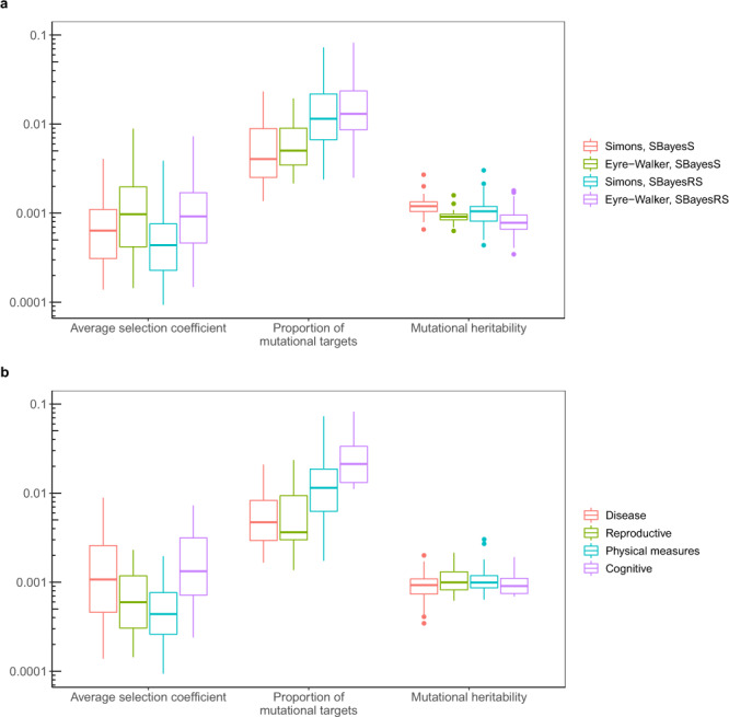
Prediction of the evolutionary parameters for 44 complex traits and diseases based on a negative selection model where selection coefficients followed a mixture distribution.

a Distribution of the predicted evolutionary parameters under different scenarios: methods used for estimating the genetic architecture parameters (SBayesS and SBayesRS) and pleiotropic effect models used for simulations (the Simons et al. and Eyre-Walker model), shown by colours. Each box plot shows the results for 44 complex traits. b Distribution of predicted evolutionary parameters for four trait categories, shown by colours. Each box plot shows the results for a number of traits in a category, with each trait having four results from analyses using different estimation methods and simulation models.

While the predicted $$ h_m^2$$ was similar across traits, the predicted $$ \overline{s}$$ and π_m were significantly different between some trait categories (Fig. 5 and Supplementary Fig. 22). Common diseases had a mean $$ \overline{s}$$ of 0.0010, which was significantly higher than that of 0.0005 for physical measures (median P value = 0.015 among the four groups of estimation methods and pleiotropic models). Compared to physical measures (mean π_m = 0.011), the mean π_m was significantly lower for disease (0.005, median P = 0.003) and was significantly higher for cognitive traits (0.023, median P = 0.017).

Analyses incorporating functional genomic annotations

The functional annotation categories used in our analysis were from the LDSC baseline model¹⁵. We excluded continuous annotations and annotations with flanking windows, resulting in 21 annotation categories such as the coding, regulatory, repressed and conserved regions (Supplementary Table 5). We applied SBayesS-strat to the 35 UKB traits (including 9 diseases), and combined the parameter estimates across traits for each functional category (see the “Methods” section). Considering the extensive overlaps between annotation categories (Supplementary Fig. 23), we ran SbayesS-strat analysis with a two-component model (SNPs in an annotation category versus the other SNPs) and computed the enrichment of each of the genetic architecture parameters using the SNPs in the focal annotation category in comparison to the genome-wide estimate using all SNPs. The fold enrichment of per-SNP heritability was correlated with that of polygenicity across annotation categories (r = 0.762; Fig. 6a). The per-SNP heritability and polygenicity were enriched in functionally important categories, such as transcription start sites (TSS), 3′- and 5′-UTRs, and conserved, enhancer and coding regions, but depleted in repressed regions. This result suggests that a functional category that explains a greater fraction of heritability tends to have a larger number of nonnull variants, consistent with the findings from a recent study¹¹. However, for some categories, such as coding and conserved regions, the fold enrichment of per-SNP heritability was greater than that of polygenicity, suggesting an enrichment of larger effect sizes in these regions. To distinguish between the contributions of the number and the magnitude of the nonzero effects to $$ h_{\mathrm{SNP}}^2$$, we estimated per-NZE heritability (per-nonzero effect heritability $$ h_{\mathrm{NZE}}^2\left(c\right)=\frac{h_{\mathrm{SNP}}^2\left(c\right)}{m_{\mathrm{NZ}}\left(c\right)}$$ where m_NZ(c) is the number of SNPs with nonzero effects in category c). While the fold enrichment of $$ h_{\mathrm{NZE}}^2\left(c\right)$$ was close to or smaller than one in most categories, the enrichment was the largest in the coding and conserved regions (Fig. 6b), suggesting that the enrichment of per-SNP heritability in these categories was not only because of the larger number of nonnull variants but also the larger effect sizes, confirmed by simulations (Supplementary Fig. 24). The median value of $$ \widehat{S}$$ was −0.540, ranging from −0.739 (s.e.m. = 0.041) in coding regions to −0.361 (s.e.m. = 0.066) in TSS (Fig. 6c). The negative $$ \widehat{S}$$ in all functional categories suggests a widespread negative selection across the whole genome, and the largest $$ ∣\widehat{S}∣$$ in the coding regions among all the functional categories highlighted the action of negative selection in the biologically most important regions.

Fig. 6

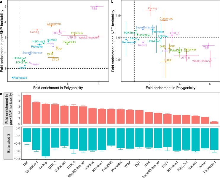
Characterisation of the genetic architecture in 21 functional genomic annotation categories using the two-component SBayesS-strat model.

a Fold enrichment of per-SNP heritability against that of polygenicity. b Fold enrichment of per-NZE (per-nonzero effect) heritability against that of polygenicity. Colours indicate different annotation categories. c Estimated S (green) across annotation categories ranked by per-SNP heritability enrichment (red). Each dot or histogram is the median across 35 UKB traits (including diseases). Each bar indicates the standard error of the mean.

Our estimates of per-SNP heritability enrichment were consistent with those from S-LDSC^15,40,41 for most annotation categories (Supplementary Fig. 25). However, S-LDSC reported a much larger enrichment for the conserved region category, followed by the coding region category. This may be due to the different assumptions made in the two methods, i.e., SBayesS-strat assumes a sparse genetic architecture whereas S-LDSC does not explicitly assume a mixture model, as both the coding and conserved regions categories were enriched for the number of nonzero effects and the magnitude of effect sizes (Fig. 6b). Another explanation could be that the SBayesS-strat estimate is from a separate analysis of a focal category at a time conditioning on all the other SNPs with no overlap among categories whereas the S-LDSC estimates are from a joint analysis of all the categories with overlaps.

SBayesS

Let us consider an individual-level data-based multiple regression model for a GWAS cohort:

When the LD correlations are computed using all SNPs in the GWAS sample, models (1) and (2) are equivalent in terms of posterior inference because the GWAS estimates of SNP effects (b) and LD correlation matrix (B) are sufficient statistics for the joint posterior distribution of β (Supplementary Note). Compared to model (1), model (2) allows us to incorporate LD information from a different reference sample from the GWAS sample for which the individual-level data are often not accessible. Further, it is often not practical to compute and store the entire LD matrix in the memory. Therefore, we used a sparse LD matrix that ignores the small LD correlation estimates due to sampling variation, but still accounted for the sampling variance of LD correlation in the model (Supplementary Note). In our GCTB software¹³ where SBayesS is implemented, we have developed a parallel computing strategy to facilitate the computation of the LD matrix. Once the LD matrix is computed, it can be used repeatedly in the GWAS summary-data analysis for different traits.

MCMC and convergence

We used MCMC algorithm to generate 50,000 posterior samples (the first 20,000 discarded as burn-in) from the joint posterior distribution of model parameters, based on which statistical inference was made. Details of the MCMC sampling scheme are shown in the Supplementary Note. The posterior mean was used as the point estimator, with the statistical uncertainty quantified by the posterior variance or its square root (posterior standard error), as shown below. We ran four parallel chains with different starting values of the parameters randomly sampled from their prior distributions. Following the method proposed by Gelman and Rubin²⁷, we estimated the posterior variance by

To assess convergence in MCMC, we computed the potential scale reduction statistic

Sparse LD matrix

For computational efficiency, we used a sparse LD matrix in the analysis where LD due to sampling variation were set to be zero. To this end, we tested whether LD between each pair of SNPs on the same chromosome is zero in the population when computing the LD correlation matrix using a reference sample. Under the null hypothesis that the true LD in the population is zero, we assume⁵¹

SNP-based heritability estimation

In BayesS¹³, we computed the genetic variance $$ {\sigma }_{\mathrm{g}}^2$$ as the variance of genetic values across individuals given the sampled values of β in each MCMC iteration. As described in Zhu and Stephens³⁵, this is equivalent to the following quadratic term of β given the LD correlation matrix:

SBayesRS

Following the recently published SBayesR²⁹ model which assumes a mixture of a point mass at zero and multiple normal distributions with different variances, we extended SBayesS to this flexible multi-component mixture model to account for a more complex genetic architecture with a spectrum of very small to very large effect sizes. For each SNP effect, we assume

SBayesS-strat

SBayesS-strat is a two-component SBayesS model that allows the distributions of SNP effects in the focal annotation category, e.g., coding, regulatory and conserved regions, to be different from that in the rest of the genome. Compared to other methods utilising functional annotations, such as S-LDSC⁵², BayesRC⁵³ and RSS-E⁵⁴, a unique feature of the annotation-stratified SBayesS (referred to as SBayesS-strat) is that it allows the estimation of S in a specific functional annotation category. Compared to a recently published method, BLD-LDAK-Alpha⁹, that estimates the S parameter (denoted by α in their model) based on an infinitesimal model, our method accounts for a sparse genetic architecture. In addition to the estimation of per-SNP heritability, polygenicity and S for each category, we also defined per-nonzero-effect (per-NZE) heritability ($$ h_{\mathrm{NZE}}^2$$) as the total heritability explained in a category divided by the number of nonzero effects in the category, which is helpful to understand whether the heritability enrichment is due to the larger number of associated variants or the larger magnitude of effect size compared to genome average. In addition to the category-specific parameters, we estimated the global parameters S, π, $$ h_{\mathrm{SNP}}^2$$ and $$ h_{\mathrm{NZE}}^2$$ empirically conditional on the sampled value of β in each iteration of MCMC. The fold of enrichment of each parameter for each trait was then computed as $$ E_{\mathrm{t}}\left[{\theta }_{\gamma }^{\mathrm{t}}/{\theta }^{\mathrm{t}}\right]$$ over T MCMC iterations. The estimation variation of the enrichment fold was quantified by the posterior variance as described above.

Meta-analysis across traits

We combined the SBayesS-strat estimates across traits by calculating the median fold enrichment for each functional category. We reported the median instead of the mean in order to minimise the impact of outliers, especially for the per-NZE heritability estimate for which the denominator (i.e., the number of nonzero effects in an annotation category) is often estimated with large sampling variance. To account for the phenotypic correlation among the traits, we estimated the effective number of traits (n_e) by performing an eigen decomposition on the phenotypic correlation matrix⁵⁵:

GWAS summary statistics

We performed GWAS analyses for 26 quantitative traits and 9 common diseases in the full release of the UKB data using PLINK 1.90 beta⁵⁶. We used 348,501 unrelated individuals of European ancestry (estimated genetic relatedness from GCTA < 0.05)⁵⁷ and the imputed data provided by the UKB team¹⁶. We filtered HapMap3 SNPs³⁰ with MAF < 0.01, HWE test P value < 1 × 10⁻⁶, missing genotype rate > 0.05, or imputation info score < 0.3. We further excluded SNPs in the Human Major Histocompatibility Complex (MHC) region, resulting in a total of 1,124,198 common SNPs for the analysis. The LD correlations in the reference samples were computed based on the effect alleles in the GWAS summary data. For quantitative traits, we standardised phenotypes to mean zero and variance one after removing the outliers (phenotype > 7 SD) and performed rank-based inverse normal transformation (RINT) within each sex group. Prior to GWAS, we pre-adjusted phenotypes by age, sex and first 10 principal components (PCs) provided by the UKB team after RINT if applied. For the publicly available summary statistics, we downloaded the data and matched the SNPs with those in the UKB data after excluding the strand ambiguous SNPs (i.e., A/T or C/G SNPs) in addition to the QC procedures above. For the GWAS summary data from the Neale Lab, we extracted 274 quantitative traits for which the GWAS was performed based on RINT phenotypes in their analysis pipeline.

Evolutionary forward simulations

We used SLiM3²⁶ to run evolutionary forward simulations. A large sequence of 100 Mb was simulated, where a proportion of new mutations (π_m) that had pleiotropic effects on fitness and trait emerged at random with an average selection coefficient of $$ \overline{s}$$ and a mutational heritability of $$ h_m^2$$ in each generation. The values of the three input parameters were sampled from uniform distributions at log10 scale: log₁₀(s) ~ U(10⁻⁵, 10⁻²), log₁₀(π_m) ~ U(10⁻³, 10⁻¹) and $$ {\log }_{10}\left(h_{\mathrm{m}}^2\right)~U\left(10^{-4},10^{-2}\right)$$. The mutation rate (μ_m) was set to 1.65 × 10⁻⁸ per base pair per individual per generation⁵⁸, and the recombination rate was set to 1 × 10⁻⁸. We assumed a model of negative selection (see below for a scenario with positive selection), where all trait variants were deleterious to fitness and the other mutations were neutral. The causal effects were assumed to have a mixture of three normal distributions with small, medium and large variances: $$ {\beta }_j~0.7N\left(0,0.01{\sigma }_{\beta }^2\right)+0.25N\left(0,0.1{\sigma }_{\beta }^2\right)+0.05N\left(0,{\sigma }_{\beta }^2\right)$$, where the mixing proportions were set to the average SBayesRS estimates across 44 real traits. Thus, the marginal variance of causal effects is $$ V_{\beta }=\mathrm{Var}\left({\beta }_j\right)=\left(0.7*0.01+0.25*0.1+0.05\right){\sigma }_{\beta }^2$$. Given the input parameters $$ h_{\mathrm{m}}^2$$ and π_m, the mixture distribution parameter $$ {\sigma }_{\beta }^2$$ can be computed because, according to population genetics theory¹⁰, $$ h_{\mathrm{m}}^2=2L{\pi }_{\mathrm{m}}{\mu }_{\mathrm{m}}{V}_{\beta }$$ in the unit of environmental variance $$ {\sigma }_e^2$$, with L being the genome length (100 Mb). For each trait mutation, the selection coefficient was modelled by $$ s_j=k{\beta }_j^2$$, where $$ k=\overline{s}/V_{\beta }$$ given the input parameter $$ \overline{s}$$. Because β_j followed a mixture distribution, s_j also followed a mixture distribution with small and large selection coefficients. To break up the perfect proportionality between selection coefficients and squared effect sizes, two pleiotropic effect models were used to remodel the trait effect of causal variant conditional on its selection coefficient toward the end of the selection process. The first model is the Simons et al.¹² model which assumes the causal effect on the focal trait (denoted as 1) following the distribution β_j1 ~ N(0, k⁻¹s_j/n_t) with n_t being the number of traits on which the variant has an effect. The second model is the Eyre-Walker’s model³: $$ {\beta }_{j1}={\delta }_j{S}_j^{\tau }\left(1+{\epsilon }_j\right)$$ with δ_j = 1 or −1 determined at random, S_j = 4N_es_j, N_e = 10,000 being the effective population size and ε_j ~ N(0, σ²). In the Eyre-Walker’s model, τ is the key parameter and σ² is a nuisance parameter. For each set of causal variants, we simulated causal effects based on either the Simons et al. model with n_t = 1, 2, 4 or 10 or the Eyre-Walker model with τ = 0.2, 0.5, 0.8, 1.0 and σ² = 0.1.

A demographic model inferred by Gravel et al.³⁷ with population bottleneck and expansion was used to simulate a population that had undergone selection for 58,000 generations. The simulation started with an ancestral base population of N_e = 7310, which was expanded to 14,474 after 52,080 generations, a long period of neutral burn-in to allow the population reach mutation-drift equilibrium (~1.3 million years assuming 25 years per generation). In generation 55,960, 1861 individuals were split from the base population into a descendant population to mimic the out-of-African dispersal. In generation 57,080, the population size was further reduced to 1032 and then increased with an exponential rate of 0.0038 until generation 58,000, reaching to a final population size of 34,039. In the last generation of selection, we obtained the genotypes of ~2000 unrelated individuals (genomic relationship < 0.05) and computed the LD correlation matrix for all common causal variants and a random sample of 36k common SNPs, a comparable density as the SNPs used in the real trait analysis (1.1 × 10⁶ × 1 × 10⁸/3 × 10⁹ = 36,000). Given the LD matrix and causal effects, we directly simulated the GWAS summary statistics for all variants^11,38: $$ \widehat{\mathit{\alpha }}~N\left(\widehat{\mathbf{B}}\mathit{\beta },\frac{1}{N}\widehat{\mathbf{B}}\right)$$, where $$ \widehat{\mathbf{B}}$$ is the LD matrix, β is the simulated causal effects based on different evolutionary models (the Simon et al. or Eyre-Walker model), and N = 350k is the sample size in the UKB dataset (see the Supplementary Note for more details). Using this approach, we were able to simulate a GWAS data set with comparable statistical power as in the real data analysis. We then used the same methods as those used in real trait analysis (i.e., SBayesS and SBayesRS) to estimate the SNP-based heritability, polygenicity and S at either common causal variants or the random set of 36,000 common SNPs (excluding the causal variants). The true value of SNP-based heritability was computed as $$ {\sigma }_{\mathrm{g}}^2/\left({\sigma }_{\mathrm{g}}^2+{\sigma }_{\mathrm{e}}^2\right)$$, where $$ {\sigma }_{\mathrm{g}}^2$$ is the genetic variance yielded from the simulation and $$ {\sigma }_{\mathrm{e}}^2=1$$. The true value for polygenicity was represented by the number of common causal variants in the last generation of selection. The true S parameter was estimated using a linear regression

To incorporate positive selection, we specified two more input parameters, i.e., proportion of trait mutations being beneficial (π_m,b) and average selection coefficient for the beneficial alleles ($$ {\overline{s}}_{\mathrm{b}}$$). Similar as above, we sampled their values from uniform distributions at log10 scale: $$ {\log }_{10}\left({\overline{s}}_{\mathrm{b}}\right)~U\left(10^{-5},10^{-2}\right)$$ and log₁₀(π_m,b) ~ U(10⁻³, 10⁻¹). In this scenario, a new mutation can either be beneficial or deleterious with a selection coefficient as modelled above given the average positive or negative selection coefficient. Note that only the Simons et al. model was used to simulate GWAS data in this scenario as the Eyre-Walker model only fits in the context of negative selection.

Inference on evolutionary parameters

We used a polynomial regression model to predict an evolutionary parameter from the estimates of the genetic architecture parameters for complex traits. The forward simulation data under either the Simons et al.¹² or Eyre-Walker³ model with various settings were used as a reference to estimate the associations between an evolutionary parameter ($$ \overline{s}$$, π_m and $$ h_{\mathrm{m}}^2$$ at log10 scale for a positive parameter space) and the genetic architecture parameters in their original units. We tested the performance of this method by a cross-validation analysis in the simulated data, with 80% of the sample as training and the rest as validation. As shown in Supplementary Fig. 20, the three evolutionary parameters, $$ \overline{s}$$, π_m and $$ h_{\mathrm{m}}^2$$, can be predicted with reasonably high accuracy, and the prediction accuracy reached the maximum when the degree of polynomial was about 3. Given this result, we chose the degree of polynomial of 3 in the real trait prediction analysis. We used the entire simulation data set to build a polynomial regression model to predict each of the evolutionary parameters by jointly modelling the SBayesS estimates of $$ h_{\mathrm{SNP}}^2,S$$ and π (or the SBayesRS estimates of $$ h_{\mathrm{SNP}}^2$$, S, π₁, π₂, π₃ and π₄). We then applied these polynomial equations to predict the evolutionary parameters in real data for 44 complex traits.

Reporting summary

Further information on research design is available in the Nature Research Reporting Summary linked to this article.