Estimation of fidelity to a coherent state

We first introduce a test scheme to estimate the fidelity between an optical state ρ and the vacuum state $$ ∣0⟩⟨0∣$$ through a heterodyne measurement. For a state ρ of a single optical mode, the heterodyne measurement produces an outcome $$ \widehat{\omega }\in \mathbb{C}$$ with a probability density

Theorem 1: Let Λ_m,r(ν) (ν ≥ 0) be a bounded function given by

From Eq. (6), a lower bound on the fidelity between ρ and the vacuum state is given by

Fig. 1

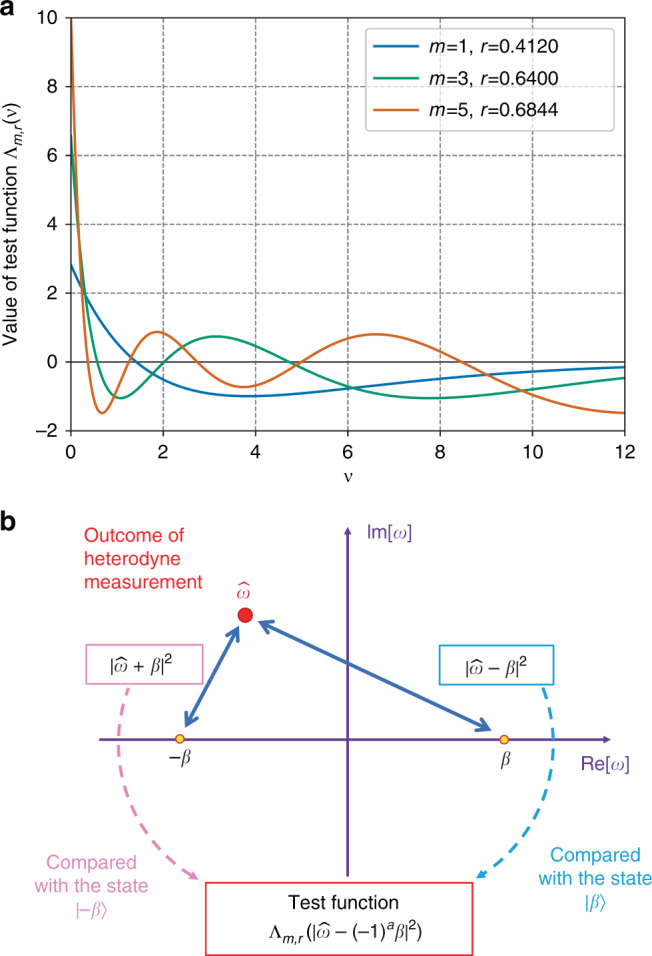
The test scheme to estimate the fidelity.

a Example of the test functions Λ_m,r used in the estimation. The values of r in the figure are chosen so that the range of Λ_m,r is minimized for given m. In general, the minimum range of the function Λ_m,r becomes larger as m increases. The pair (m, r) = (1, 0.4120) was used in the numerical simulation of key rates below. b A schematic description of the usage of obtained outcomes in heterodyne measurement. In order to estimate the lower bound on the fidelity to the coherent states $$ ∣\pm \beta ⟩$$, the squared distance between the outcome $$ \widehat{\omega }$$ and the objective point (−1)^aβ (i.e., $$ \mid \widehat{\omega }-{\left(-1\right)}^a\beta {\mid }^2$$) is used.

Extension to the fidelity to a coherent state $$ ∣\beta ⟩$$ is straightforward as

Proposed protocol

Based on this fidelity test, we propose the following discrete-modulation protocol (see Fig. 2). Prior to the protocol, Alice and Bob determine the number of rounds N, the acceptance probability of homodyne measurement $$ f_{\mathrm{suc}}\left(\mid x\mid \right)\left(x\in \mathbb{R}\right)$$ with f_suc(0) = 0, the parameters for the test function (m, r), and the protocol parameters (μ, p_sig, p_test, p_trash, β, s) with p_sig + p_test + p_trash = 1, where all the parameters are positive. Alice and Bob then run the protocol described in Box 1. Upon successful verification, the protocol generates a shared final key of length

Fig. 2

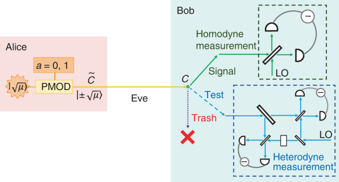
The proposed continuous-variable quantum key distribution protocol.

Alice generates a random bit a ∈ {0, 1} and sends a coherent state with amplitude $$ {\left(-1\right)}^a\sqrt{\mu }$$. Bob chooses one of the three measurements based on the predetermined probability. In the signal round, Bob performs a homodyne measurement on the received optical pulse and obtains an outcome $$ \widehat{x}$$. In the test round, Bob performs a heterodyne measurement on the received optical pulse and obtains an outcome $$ \widehat{\omega }$$. In the trash round, he produces no outcome.

The acceptance probability f_suc(∣x∣) should be chosen to post-select the rounds with larger values of ∣x∣, for which the bit error probability is expected to be lower. It is ideally a step function, but our security proof is applicable to any form of f_suc(∣x∣). The parameter β is typically chosen to be $$ \sqrt{\eta \mu }$$ with η being a nominal transmissivity of the quantum channel, while the security proof itself holds for any choice of β. The parameters s and $$ s^{\prime }$$ are related to the overall security parameter in the security proof below.

Security proof

We determine a sufficient amount of the privacy amplification according to Shor and Preskill^37,40, which has been widely used for the DV-QKD protocols. We consider a coherent version of Steps 1 and 2, in which Alice and Bob share an entangled pair of qubits for each success signal round, such that their Z-basis measurement outcomes correspond to the sifted key bits a and b. For Alice, we introduce a qubit A and assume that she entangles it with an optical pulse $$ \tilde{C}$$ in a state

Fig. 3

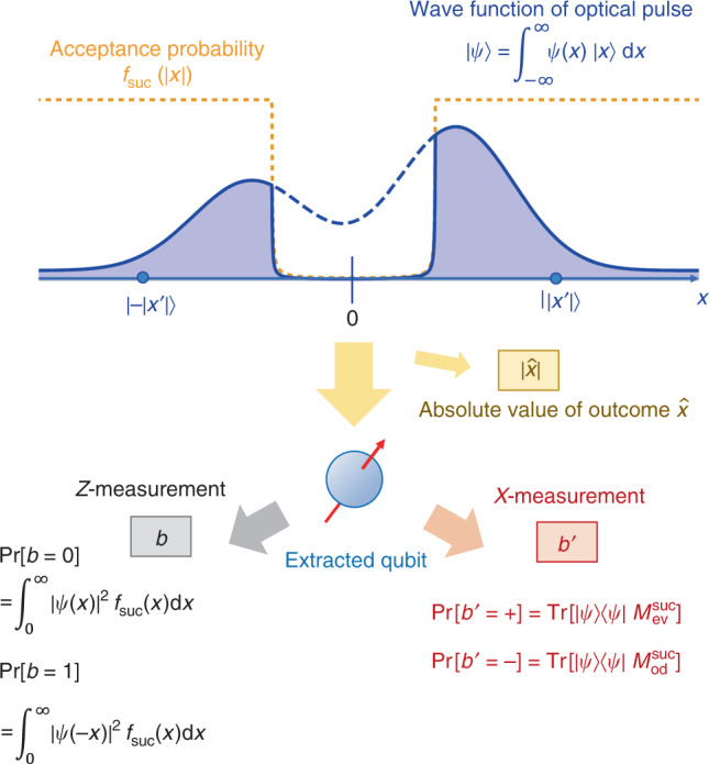
Bob’s qubit extraction in the entanglement-sharing protocol.

Bob performs on the optical pulse a non-demolition projective measurement, with which the absolute value of the outcome of homodyne measurement $$ \mid \widehat{x}\mid $$ is determined. Then, Bob extracts a qubit B by the operation $$ \mathcal{F}$$ defined in Eq. (11). A Z-basis measurement on this qubit gives the same sifted key bit b as described in the actual protocol. On the other hand, the X-basis measurement on this qubit reveals the parity of photon number of the received optical pulse.

To clarify the above observation, we introduce an entanglement-sharing protocol defined in Box 2. This protocol leaves $$ {\widehat{N}}^{\mathrm{suc}}$$ pairs of qubits shared by Alice and Bob. If they measure these qubits on Z basis to define the sifted key bits, the whole procedure is equivalent to Steps 1 through 3 of the actual protocol (see Fig. 4). Alice’s measurements on X basis $$ \left\{∣\pm ⟩:=\left(∣0⟩+∣1⟩\right)/\sqrt{2}\right\}$$ in the trash rounds are added for later security argument, and they do not affect the equivalence.

Fig. 4

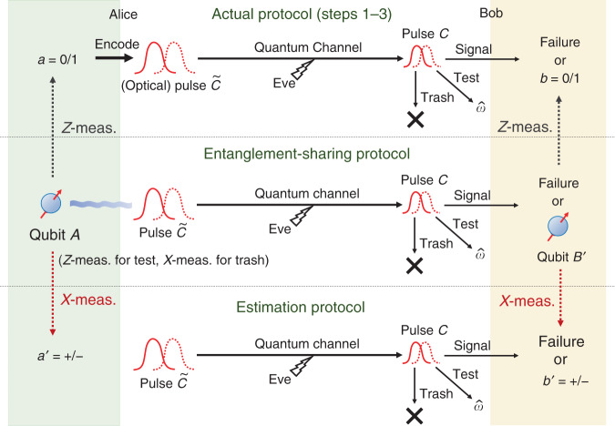
Relation between three protocols.

The actual protocol and the estimation protocol are related through the entanglement-sharing protocol. After the entanglement-sharing protocol, Alice and Bob are left with the observed data $$ \left({\widehat{N}}^{\mathrm{suc}},{\widehat{N}}^{\mathrm{fail}},{\widehat{N}}^{\mathrm{test}},{\widehat{N}}^{\mathrm{trash}},\widehat{F},{\widehat{Q}}_{-}\right)$$ and $$ {\widehat{N}}^{\mathrm{suc}}$$ pairs of qubits. If Alice and Bob ignore $$ {\widehat{Q}}_{-}$$ and measure their qubits on the Z-basis to determine their $$ {\widehat{N}}^{\mathrm{suc}}$$-bit sifted keys, it becomes equivalent to the actual protocol. On the other hand, if Alice and Bob measure their $$ {\widehat{N}}^{\mathrm{suc}}$$ pairs of qubits on the X-basis, they can count the number $$ {\widehat{N}}_{\mathrm{ph}}^{\mathrm{suc}}$$ of phase errors, which we call the estimation protocol. If we can find a reliable upper bound U on $$ {\widehat{N}}_{\mathrm{ph}}^{\mathrm{suc}}$$ in the estimation protocol, it restricts the property of the state of $$ {\widehat{N}}^{\mathrm{suc}}$$ pairs of qubits after the entanglement-sharing protocol, which in turn limits the amount of leaked information on the sifted keys in the actual protocol. The security proof is thus reduced to finding such an upper bound U in the estimation protocol, represented as a function of the variables that are commonly available in the three protocols.

The Shor-Preskill argument connects the amount of privacy amplification to the so-called phase error rate. Suppose that, after the entanglement-sharing protocol, Alice and Bob measure their $$ {\widehat{N}}^{\mathrm{suc}}$$ pairs of qubits on X basis $$ \left\{∣+⟩,∣-⟩\right\}$$. A pair with outcomes (+, −) or (−, +) is defined to be a phase error. Let $$ {\widehat{N}}_{\mathrm{ph}}^{\mathrm{suc}}$$ be the number of phase errors among $$ {\widehat{N}}^{\mathrm{suc}}$$ pairs. If we can have a good upper bound e_ph on the phase error rate $$ {\widehat{N}}_{\mathrm{ph}}^{\mathrm{suc}}/{\widehat{N}}^{\mathrm{suc}}$$, shortening by fraction h(e_ph) via privacy amplification in the actual protocol achieves the security in the asymptotic limit³⁷.

To cover the finite-size case as well, we need a more rigorous statement on the upper bound. For that purpose, we define an estimation protocol in Box 3 (see also Fig. 4). The task of proving the security of the actual protocol is then reduced to construction of a function $$ U\left(\widehat{F},{\widehat{N}}^{\mathrm{trash}}\right)$$ which satisfies

At this point, it is beneficial for the analysis of the phase error statistics to clarify what property of the optical pulse C is measured by Bob’s X-basis measurement in the estimation protocol (see Fig. 3). Let Π_ev(od) be the projection to the subspace with even (resp. odd) photon numbers. (Π_ev + Π_od = 1_C holds by definition.) Furthermore, since Π_ev − Π_odd is the operator for an optical phase shift of π, we have $$ \left({\mathrm{\Pi }}_{\mathrm{ev}}-{\mathrm{\Pi }}_{\mathrm{odd}}\right)∣x⟩=∣-x⟩$$. Eq. (12) is then rewritten as

As an intermediate step toward our final goal of Eq. (15), let us first derive a bound on the expectation value $$ \mathbb{E}\left[{\widehat{N}}_{\mathrm{ph}}^{\mathrm{suc}}\right]$$ in terms of those collected in the test and the trash rounds, $$ \mathbb{E}\left[\widehat{F}\right]$$ and $$ \mathbb{E}\left[{\widehat{Q}}_{-}\right]$$, in the estimation protocol. Let ρ_AC be the state of the qubit A and the received pulse C averaged over N pairs, and define relevant operators as

It is expected that a meaningful bound is obtained only for κ, γ ≥ 0. Decreasing fidelity $$ ⟨{\mathrm{\Pi }}^{\mathrm{fid}}⟩$$ should allow more room for eavesdropping, leading to a larger value of phase error rate $$ ⟨M_{\mathrm{ph}}^{\mathrm{suc}}⟩$$. Hence Eq. (25) will give a good bound only when κ≥0. As for $$ ⟨{\mathrm{\Pi }}_{-}^{\mathrm{trash}}⟩$$, it only depends on the marginal state of Alice’s qubit A, which is independent of the adversary’s attack. We thus have $$ ⟨{\mathrm{\Pi }}_{-}^{\mathrm{trash}}⟩=q_{-}:={∥{⟨-∣}_A{∣\mathrm{\Psi }⟩}_{A\tilde{C}}∥}^2=\left(1-e^{-2\mu }\right)/2$$. Since Alice’s use of a stronger pulse should lead to larger leak of information, we should choose γ ≥ 0 for a good bound.

To find a function B(κ, γ) satisfying Eq. (25), let us define an operator

With B(κ, γ) computed, we can rewrite Eq. (25) using Eqs. (22)–(24) to obtain a relation between $$ \mathbb{E}\left[{\widehat{N}}_{\mathrm{ph}}^{\mathrm{suc}}\right]$$, $$ \mathbb{E}\left[\widehat{F}\right]$$, and $$ \mathbb{E}\left[{\widehat{Q}}_{-}\right]$$. It is concisely written as

The security in the finite-size regime is proved as follows. The fact that the bound given in Eq. (28) is true for all the states ρ_AC allows us to use Azuma’s inequality⁴² to evaluate the fluctuations around the expectation value, leading to an inequality

Although Eq. (29) includes $$ {\widehat{Q}}_{-}$$ which is inaccessible in the actual protocol, we can derive a bound by noticing that it is an outcome from Alice’s qubits and is independent of the adversary’s attack. In fact, given $$ {\widehat{N}}^{\mathrm{trash}}$$, it is the tally of $$ {\widehat{N}}^{\mathrm{trash}}$$ Bernoulli trials with a probability q₋. Hence, we can derive an inequality of the form

Numerical simulation

We simulated the net key gain per pulse $$ \widehat{G}$$ as a function of attenuation in the optical channel (including the efficiency of Bob’s apparatus). We assume a channel model with a loss with transmissivity η and an excess noise at channel output; Bob receives Gaussian states obtained by randomly displacing coherent states $$ ∣\pm \sqrt{\eta \mu }⟩$$ to increase their variances by a factor of (1 + ξ)^43,44. We assume a step function with a threshold x_th( > 0) as the acceptance probability f_suc(∣x∣). The expected amplitude of coherent state β is chosen to be $$ \sqrt{\eta \mu }$$. We set $$ {ϵ}_{\sec }=2^{-50}$$ for the security parameter, and set $$ ϵ=2^{-s}={ϵ}_{\sec }^2/16$$ and $$ 2^{-s^{\prime }}={ϵ}_{\sec }/2$$. We thus have two coefficients (κ, γ), four protocol parameters (μ, x_th, p_sig, p_test), and two parameters (m, r) of the test function to be determined. For each transmissivity η, we determined (κ, γ) via a convex optimization using the CVXPY 1.0.25^45,46 and (μ, x_th, p_sig, p_test) via the Nelder-Mead in the scipy.minimize library in Python, in order to maximize the key rate. Furthermore, we adopted m = 1 and r = 0.4120, which leads to $$ \left(\max {\mathrm{\Lambda }}_{m,r},\min {\mathrm{\Lambda }}_{m,r}\right)=\left(2.824,-0.9932\right)$$. See Methods for the detail of the model of our numerical simulation and examples of optimized parameters. Typical optimized values of the threshold x_th range from 0.4 to 1.5 (we adopted a normalization for which the vacuum fluctuation is $$ \sqrt{⟨{\left(\mathrm{\Delta }x\right)}^2⟩}=0.5$$). They are larger than those in other analyses of protocols with post-selection (e.g., ref. ³¹). A possible reason is the fact that the latter protocols use more than two states to monitor the eavesdropping act, which may lead to a lower cost of privacy amplification and higher tolerance against bit errors.

Figure 5 shows the key rates of our protocol in the asymptotic limit N → ∞ and finite-size cases with N = 10⁹–10¹² for ξ = 10^−2.0–10^−3.0 and 0. (Note that from the results of the recent experiments^8,44,47, excess noise with ξ = 10^−2.0–10^−3.0 at the channel output seems reasonable. Furthermore, the state-of-the-art experiments⁸ work at 0.5 GHz repetition rate, which implies that total number of rounds N = 10⁹–10¹² can be achieved in a realistic duration.) For the noiseless model (ξ = 0), the asymptotic rate reaches 8 dB. In the case of ξ = 10^−3.0, it reaches 4 dB, which is comparable to the result of a similar binary modulation protocol proposed in ref. ²⁹. As for finite-size key rates, we see that the noiseless model shows a significant finite-size effect even for N = 10¹². On the other hand, with a presence of noises (ξ = 10^−3.0) the effect becomes milder, and N = 10¹¹ is enough to achieve a rate close to the asymptotic case. This may be ascribed to the cost of the fidelity test. In order to make sure that the fidelity is no smaller than 1 − δ, the statistical uncertainty of the fidelity test must be reduced to O(δ). As a result, approaching the asymptotic rate of ξ = 0 will require many rounds for the fidelity test.

Fig. 5

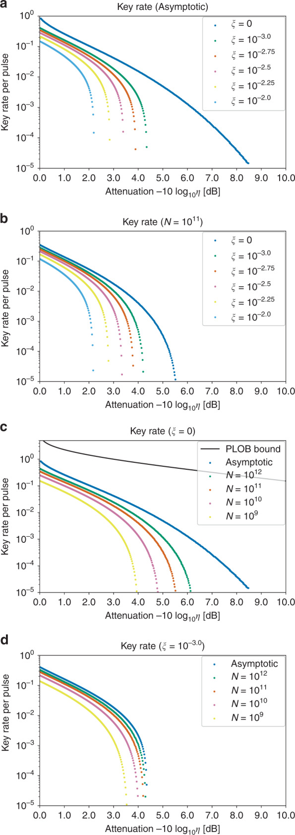
The net key gain per pulse $$ \widehat{G}$$ (key rate) vs. transmissivity η of the optical channel.

The abscissa represents attenuation in decibel, i.e., $$ -10{\log }_{10}\eta $$. We assumed that the optical pulse that Bob receives is given by randomly displacing a coherent state to increase its variance by a factor of (1 + ξ). a The asymptotic key rate for various values of ξ. b The key rate for various values of ξ when the pulse number is finite (N = 10¹¹). c The key rate without the excess noise (ξ = 0) along with the repeaterless bound (PLOB bound) of the secure key rate in the pure-loss channel⁵⁵. d The key rate with the excess noise of ξ = 10^−3.0.

Proof of Theorem 1 and Eq. (8)

In this section, we prove Theorem 1 stated in the main text and derive Eq. (8) as a corollary of Theorem 1.

Proof: From Eq. (1), the expectation value of $$ {\mathrm{\Lambda }}_{m,r}\left(\mid \widehat{\omega }{\mid }^2\right)$$ when given a measured state ρ is given by

The following three properties hold for I_n,m:

(i)I_n,m = 0 for m ≥ n ≥ 1.

This results from orthogonality relations of the associated Laguerre polynomials, that is,

(ii)(−1)^mI_n,m > 0 for n > m ≥ 0.

This property is shown as follows. First, the associated Laguerre polynomials satisfy the following recurrence relation for m ≥ 1⁴⁹:

(iii)I_0,m = 1 for m ≥ 0.

This also follows from property (i) and Eq. (36) for n = 1 and m ≥ 1, which leads to I_0,m = I_0,0 = 1.

Combining properties (i), (ii), and (iii) shows Eq. (6).

Eq. (8) in the main text is derived as the following corollary.

Corollary 1: Let $$ ∣\beta ⟩$$$$ \left(\beta \in \mathbb{C}\right)$$ be the coherent state with amplitude β. Then, for any $$ \beta \in \mathbb{C}$$ and for any odd positive integer m, we have

Proof: From Eq. (6) of Theorem 1, for any odd positive integer m, we have

Detail of the security proof

In this section, we prove the security of the proposed protocol in the main text. This section consists of several subsections. In the first subsection, we give a definition of security, which is standard in the literature. The security condition is divided into two conditions, secrecy and correctness. Since the correctness is trivially satisfied, it is the secrecy that is the focus of the security proof. The second subsection explains how the secrecy condition is reduced to Eq. (15) of the estimation protocol, which bounds the number of phase errors. The third subsection lays the groundwork for the full security proof by deriving the inequality (27) involving three operators relevant for the quantities observed in the signal, the test, and the trash round in the estimation protocol. After proving a general lemma (Lemma 1), an explicit form of the upper bound B(κ, γ) satisfying Eq. (27) is given as a corollary (Corollary 2) of the lemma. Finally, the fourth subsection uses Azuma’s inequality and Corollaries 1 and 2 to derive an explicit form of $$ U\left(\widehat{F},{\widehat{N}}^{\mathrm{trash}}\right)$$ that fulfills Eq. (15), which completes the security proof of the actual protocol.

1. Definition of security in the finite-size regime. We evaluate the secrecy of the final key as follows. When the final key length is N^fin ≥ 1, we represent Alice’s final key and an adversary’s quantum system as a joint state

For correctness, we say a protocol is ϵ_cor-correct if the probability for Alice’s and Bob’s final key to differ is bounded by ϵ_cor. Our protocol achieves $$ {ϵ}_{\mathrm{cor}}=2^{-s^{\prime }}$$ via the verification in Step 4.

When the above two conditions are met, the protocol becomes $$ {ϵ}_{\sec }$$-secure with $$ {ϵ}_{\sec }={ϵ}_{\mathrm{sct}}+{ϵ}_{\mathrm{cor}}$$ in the sense of universal composability⁵⁰.

2. Reduction to the estimation protocol. Here we show that Eq. (15) in the estimation protocol implies ϵ_sct-secrecy of the actual protocol with $$ {ϵ}_{\mathrm{sct}}=\sqrt{2}\sqrt{ϵ+2^{-s}}$$. We have already seen that the entanglement-sharing protocol immediately followed by Z-basis measurements of the qubits is equivalent to Steps 1 through 3 of the actual protocol. Here we consider a slightly modified scenario in which, after the entanglement-sharing protocol, a controlled-NOT operation V is applied on each pair of qubits, where $$ V:=∣0⟩{⟨0∣}_A\otimes {\mathbf{1}}_B+∣1⟩{⟨1∣}_A\otimes X_B$$ with $$ X_B:=∣1⟩{⟨0∣}_B+∣0⟩{⟨1∣}_B$$. Alice then measures her qubits on the Z basis to define her sifted key bits and proceeds with Step 5 of the actual protocol. Since V does not affect the Z-basis value of the Alice’s qubit, her procedure of determining the $$ {\widehat{N}}^{\mathrm{fin}}$$-bit final key in this scenario is equivalent to that in the actual protocol. Although V prevents Bob from obtaining an equivalent final key, he can still simulate the reconciliation and the verification process in Step 4 since the Z-basis value of each of his $$ {\widehat{N}}^{\mathrm{suc}}$$ qubits corresponds to absence/presence of a bit error between Alice’s and Bob’s sifted key bits. Hence Bob can equivalently carry out all the announcements in Steps 4 and 5 of the actual protocol. As a result, this scenario leads to exactly the same distribution Pr(N^fin) and the same states $$ {\rho }_{\mathrm{AE}\mid N^{\mathrm{fin}}}^{\mathrm{fin}}$$ as those of the actual protocol.

The secrecy of Alice’s final key can be determined from the X-basis property of her $$ {\widehat{N}}^{\mathrm{suc}}$$ qubits after the application of V. Since V can be rewritten as $$ V={\mathbf{1}}_A\otimes ∣+⟩{⟨+∣}_B+Z_A\otimes ∣-⟩{⟨-∣}_B$$ with $$ Z_A:=∣-⟩{⟨+∣}_A+∣+⟩{⟨-∣}_A$$, the X-basis value of each of Alice’s qubits corresponds to absence/presence of a phase error. Suppose that these $$ {\widehat{N}}^{\mathrm{suc}}$$ qubits are measured on the X-basis to produce an outcome $$ \widehat{\mathit{x}}\in {\left\{+,-\right\}}^{{\widehat{N}}^{\mathrm{suc}}}$$. Let $$ \mathrm{wt}\left(\widehat{\mathit{x}}\right)$$ be the number of symbol ‘−’ in $$ \widehat{\mathit{x}}$$. If Eq. (15) holds in the estimation protocol, the statistics of $$ \widehat{\mathit{x}}$$ should satisfy

We remark that the encryption of $$ M:=H_{\mathrm{EC}}+s^{\prime }$$ bits in Step 4 can be omitted as long as each bit linearly depends on Alice’s sifted key over GF(2). In such a case, the above scenario must include measurements on Alice’s qubits to simulate the announcement of the M bits in Step 4. The backaction on X basis caused by the measurement for each bit amounts to doubling the number of probable patterns $$ \widehat{\mathit{x}}$$. We can thus redefine the set $$ \mathcal{T}\left({\widehat{N}}^{\mathrm{suc}},\widehat{F},{\widehat{N}}^{\mathrm{trash}}\right)$$ by enlarging its size by factor of 2^M such that Eq. (45) holds. Then, by decreasing $$ {\widehat{N}}^{\mathrm{fin}}$$ by M, Eq. (46) also holds. This means that we achieve the same net key rate with the same level of security.

3. Derivation of the operator inequality. The aim of this subsection is to construct B(κ, γ) which fulfills the operator inequality (27). Let $$ {\sigma }_{\sup }\left(O\right)$$ denote the supremum of the spectrum of a bounded self-adjoint operator O. Although $$ B\left(\kappa ,\gamma \right)={\sigma }_{\sup }\left(M\left[\kappa ,\gamma \right]\right)$$ would give the tightest bound satisfying Eq. (27), it is hard to compute it numerically since system C has an infinite-dimensional Hilbert space. Instead, we derive a looser but simpler bound. We first prove the following lemma.

Lemma 1: Let Π_± be orthogonal projections satisfying Π₊Π₋ = 0. Suppose that the rank of Π_± is no smaller than 2 or infinite. Let M_± be self-adjoint operators satisfying Π_±M_±Π_± = M_± ≤ α_±Π_±, where α_± are real constants. Let $$ ∣\psi ⟩$$ be an unnormalized vector satisfying $$ \left({\mathrm{\Pi }}_{+}+{\mathrm{\Pi }}_{-}\right)∣\psi ⟩=∣\psi ⟩$$ and $$ {\mathrm{\Pi }}_{\pm }∣\psi ⟩\ne 0$$. Define following quantities with respect to $$ ∣\psi ⟩$$:

Proof: We choose orthonormal vectors $$ \left\{∣e_{\pm }^{\left(1\right)}⟩,∣e_{\pm }^{\left(2\right)}⟩\right\}$$ in the domain of Π_±, respectively, to satisfy

As a corollary, we derive Eq. (27) as follows.

Corollary 2: Let $$ ∣\beta ⟩$$ be a coherent state. Let Π_ev(od), $$ M_{\mathrm{ev}\left(\mathrm{od}\right)}^{\mathrm{suc}}$$, and M[κ, γ] be as defined in the main text, and define following quantities:

Proof: Let us first observe that the operator Π^fid defined in Eq. (20) can be rewritten as follows:

4. Derivation of the finite-size bound. Here we construct the function $$ U\left(\widehat{F},{\widehat{N}}^{\mathrm{trash}}\right)$$ to satisfy Eq. (15) in the estimation protocol. For that, we will first derive Eq. (30). In the estimation protocol, we define the following random variables labeled by the number i of the round;

(i)$$ {\widehat{N}}_{\mathrm{ph}}^{\mathrm{suc},\left(i\right)}$$ is defined to be unity only when “signal” is chosen in the i-th round, the detection is a “success”, and a pair of outcomes $$ \left(a^{\prime },b^{\prime }\right)$$ is (+, −) or (−, +). Otherwise, $$ {\widehat{N}}_{\mathrm{ph}}^{\mathrm{suc},\left(i\right)}=0$$. We have


and $$ {\widehat{N}}_{\mathrm{ph}}^{\mathrm{suc}}={\sum }_{i=1}^N{\widehat{N}}_{\mathrm{ph}}^{\mathrm{suc},\left(i\right)}$$.

(ii)$$ {\widehat{F}}^{\left(i\right)}$$ is defined to be $$ {\mathrm{\Lambda }}_{m,r}\left(\mid \widehat{\omega }-{\left(-1\right)}^a\beta {\mid }^2\right)$$ when “test” is chosen in the i-th round. We have


and $$ \widehat{F}={\sum }_{i=1}^N{\widehat{F}}^{\left(i\right)}$$.

(iii)$$ {\widehat{Q}}_{-}^{\left(i\right)}$$ is defined to be unity only when “trash” is chosen in the i-th round and $$ a^{\prime }=-$$. Otherwise, $$ {\widehat{Q}}_{-}^{\left(i\right)}=0$$. We have


and $$ {\widehat{Q}}_{-}={\sum }_{i=1}^N{\widehat{Q}}_{-}^{\left(i\right)}$$.

(iv)We also define


which leads to $$ \widehat{T}\left[\kappa ,\gamma \right]={\sum }_{i=1}^N{\widehat{T}}^{\left(i\right)}$$.

We will make use of Azuma’s inequality⁴². We define stochastic processes $$ {\left\{{\widehat{X}}^{\left(k\right)}\right\}}_{k=0,\dots ,N}$$ and $$ {\left\{{\widehat{Y}}^{\left(k\right)}\right\}}_{k=1,\dots ,N}$$ as follows:

Proposition 1 (Azuma’s inequality^52,53): Suppose $$ {\left\{{\widehat{X}}^{\left(k\right)}\right\}}_{k=0,1,\dots }$$ is a martingale which satisfies

We define constants $$ c_{\min }$$ and $$ c_{\max }$$ as follows. In each round, at most one of $$ {\widehat{N}}_{\mathrm{ph}}^{\mathrm{suc},\left(i\right)}$$, $$ {\widehat{F}}^{\left(i\right)}$$, and $$ {\widehat{Q}}_{-}^{\left(i\right)}$$ takes non-zero value; $$ {\widehat{N}}_{\mathrm{ph}}^{\mathrm{suc},\left(i\right)}$$ and $$ {\widehat{Q}}_{-}^{\left(i\right)}$$ are either zero or unity, and $$ \min {\mathrm{\Lambda }}_{m,r}\le {\widehat{F}}^{\left(i\right)}\le \max {\mathrm{\Lambda }}_{m,r}$$. Since κ, γ ≥ 0, Eq. (95) holds when $$ c_{\min }$$ and $$ c_{\max }$$ are defined as

Next, we will construct a deterministic bound on $$ {\widehat{Y}}^{\left(i\right)}$$. Let $$ {\rho }_{AC}^{\left(i\right)}$$ be the state of Alice’s i-th qubit and Bob’s i-th pulse conditioned on $$ {\widehat{X}}^{<i}$$. Then, using the same argument as that has lead to Eqs. (22)–(24), we have

The function $$ {\delta }_2\left(ϵ/2;{\widehat{N}}^{\mathrm{trash}}\right)$$ satisfying the bound (31) on $$ {\widehat{Q}}_{-}$$ can be derived from the fact that $$ \mathrm{Pr}\left[{\widehat{Q}}_{-}\mid {\widehat{N}}^{\mathrm{trash}}\right]$$ is a binomial distribution. The following inequality thus holds for any positive integer n and a real δ with 0 < δ < (1 − q₋)n (Chernoff bound):

Combining Eq. (30) and Eq. (31), we obtain Eq. (15) by setting

Models for numerical simulation of key rates

In what follows, we normalize quadrature x such that a coherent state $$ ∣\omega ⟩$$ has expectation $$ ⟨x⟩=\mathrm{Re}\left(\omega \right)$$ and variance $$ ⟨{\left(\mathrm{\Delta }x\right)}^2⟩=1/4$$. The wave function for ω = ω_R + iω_I is given by

For the simulation of the key rate $$ \widehat{G}$$, we assume that the communication channel and Bob’s detection apparatus can be modeled by a pure loss channel followed by random displacement, that is, the states which Bob receives are given by

We assume that Bob sets $$ \beta =\sqrt{\eta \mu }$$ for the fidelity test. The actual fidelity between Bob’s objective state $$ ∣{\left(-1\right)}^a\sqrt{\eta \mu }⟩$$ and the model state $$ {\rho }_{\mathrm{model}}^{\left(a\right)}$$ is given by

We assume that the number of “success” signal rounds $$ {\widehat{N}}^{\mathrm{suc}}$$ is equal to its expectation value,

Under these assumptions, the key rate $$ \widehat{G}$$ for each transmissivity η is optimized over two coefficients (κ, γ) and four protocol parameters (μ, x_th, p_sig, p_test) as discussed in the main part. Examples of optimized parameters are shown in Table 1. The cost of bit error correction H_EC is assumed to be $$ 1.1\times {\widehat{N}}^{\mathrm{suc}}h\left(e_{\mathrm{bit}}\right)$$, where the bit error rate e_bit is given by

Table 1

Examples of optimized parameters.

η [dB]	Key rate $$ \widehat{G}$$	(κ, γ)	μ	xth	psig	ptest
Parameters for N = 1011 and ξ = 0
0.5	2.17 × 10−1	(44.9, 1.92)	0.554	0.451	0.821	0.172
1.0	1.38 × 10−1	(32.4, 1.38)	0.514	0.532	0.821	0.172
1.5	8.71 × 10−2	(24.9, 1.01)	0.487	0.610	0.816	0.176
2.0	5.36 × 10−2	(20.3, 0.741)	0.442	0.724	0.831	0.160
2.5	3.16 × 10−2	(17.0, 0.538)	0.459	0.771	0.788	0.205
3.0	1.75 × 10−2	(14.6, 0.381)	0.451	0.855	0.767	0.227
3.5	8.92 × 10−3	(13.6, 0.262)	0.446	0.941	0.706	0.289
4.0	4.15 × 10−3	(12.6, 0.175)	0.442	1.03	0.624	0.371
4.5	1.50 × 10−3	(11.4, 0.107)	0.439	1.13	0.522	0.473
5.0	3.23 × 10−4	(9.98, 0.059)	0.438	1.25	0.370	0.626
5.5	1.63 × 10−5	(8.78, 0.031)	0.443	1.37	0.126	0.869
Parameters for N = 1011 and ξ = 10−3.0
0.5	1.79 × 10−1	(23.5, 1.60)	0.491	0.489	0.854	0.137
1.0	1.13 × 10−1	(17.9, 1.19)	0.466	0.567	0.853	0.138
1.5	6.95 × 10−2	(14.3, 0.889)	0.450	0.645	0.848	0.143
2.0	4.07 × 10−2	(11.9, 0.666)	0.442	0.724	0.831	0.160
2.5	2.20 × 10−2	(10.1, 0.487)	0.439	0.808	0.804	0.187
3.0	1.02 × 10−2	(8.85, 0.345)	0.440	0.898	0.758	0.233
3.5	3.56 × 10−3	(7.72, 0.232)	0.447	0.999	0.674	0.316
4.0	5.29 × 10−4	(6.70, 0.147)	0.463	1.11	0.484	0.505
Parameters for N = 1012 and ξ = 0
0.5	2.68 × 10−1	(82.9, 2.26)	0.616	0.421	0.864	0.133
1.0	1.69 × 10−1	(54.9, 1.56)	0.556	0.504	0.874	0.123
1.5	1.08 × 10−1	(40.3, 1.11)	0.518	0.590	0.873	0.124
2.0	6.76 × 10−2	(31.3, 0.798)	0.493	0.670	0.868	0.128
2.5	4.12 × 10−2	(26.5, 0.575)	0.475	0.750	0.852	0.145
3.0	2.41 × 10−2	(23.2, 0.408)	0.466	0.834	0.829	0.168
3.5	1.32 × 10−2	(20.1, 0.275)	0.449	0.919	0.803	0.195
4.0	6.93 × 10−3	(17.7, 0.184)	0.443	1.01	0.772	0.226
4.5	3.15 × 10−3	(16.4, 0.115)	0.434	1.10	0.698	0.300
5.0	1.14 × 10−3	(14.6, 0.065)	0.427	1.21	0.596	0.402
5.5	3.29 × 10−4	(12.9, 0.036)	0.423	1.32	0.467	0.531
6.0	3.23 × 10−5	(10.8, 0.017)	0.421	1.45	0.240	0.759
Parameters for N = 1012 and ξ = 10−3.0
0.5	2.09 × 10−1	(29.4, 1.71)	0.513	0.474	0.906	0.089
1.0	1.32 × 10−1	(21.7, 1.25)	0.482	0.554	0.909	0.086
1.5	8.23 × 10−2	(16.9, 0.928)	0.462	0.633	0.909	0.086
2.0	4.92 × 10−2	(13.8, 0.689)	0.450	0.712	0.899	0.096
2.5	2.74 × 10−2	(11.5, 0.502)	0.444	0.797	0.888	0.107
3.0	1.36 × 10−2	(9.82, 0.355)	0.442	0.886	0.858	0.137
3.5	5.28 × 10−3	(8.26, 0.237)	0.446	0.989	0.834	0.161
4.0	1.17 × 10−3	(7.13, 0.151)	0.458	1.10	0.701	0.293